16.5 CONSTRAINT SPACE DIAGRAM AND DEGREE OF WAVE PIPELINING
If the setup/hold times are ignored, the constraints expressed in (16.11) and (16.12) can be expressed as
![]()
and
![]()
The plot of these equations as a function of Δ and Tclk is referred to as the timing constraint space diagram and is shown in Fig. 16.21. The parameter k is referred to as the degree of wave pipelining. It is clear from the figure that for fixed values of k, distinct feasible regions of operation are available.
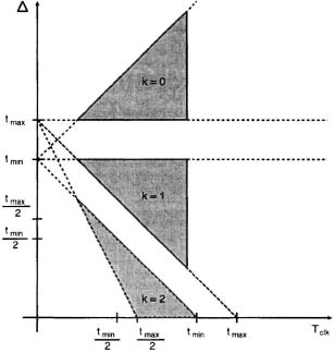
Fig. 16.21 Constraint space diagram.
Furthermore, as k is increased, the feasible region is reduced. Special values of k and Δ are interesting from a design point of view. In the following, these cases are analyzed and their effect on the clock period is also studied. The analysis is performed by using the simplified constraints of (16.22) and (16.23).
16.5.1 Δ ≤ Tclk
This constraint forces the designer to operate in the highest k region to achieve a low clock period. The simplified constraints of (16.22) and (16.23) can be expressed equivalently as
![]()
and
The problem definition results in the additional ...
Get VLSI Digital Signal Processing Systems: Design and Implementation now with the O’Reilly learning platform.
O’Reilly members experience books, live events, courses curated by job role, and more from O’Reilly and nearly 200 top publishers.

