Chapter 4. Working with Key/Value Pairs
This chapter covers how to work with RDDs of key/value pairs, which are a common data type required for many operations in Spark. Key/value RDDs are commonly used to perform aggregations, and often we will do some initial ETL (extract, transform, and load) to get our data into a key/value format. Key/value RDDs expose new operations (e.g., counting up reviews for each product, grouping together data with the same key, and grouping together two different RDDs).
We also discuss an advanced feature that lets users control the layout of pair RDDs across nodes: partitioning. Using controllable partitioning, applications can sometimes greatly reduce communication costs by ensuring that data will be accessed together and will be on the same node. This can provide significant speedups. We illustrate partitioning using the PageRank algorithm as an example. Choosing the right partitioning for a distributed dataset is similar to choosing the right data structure for a local one—in both cases, data layout can greatly affect performance.
Motivation
Spark provides special operations on RDDs containing key/value pairs.
These RDDs are called pair RDDs.
Pair RDDs are a useful building block in many programs, as they expose operations that allow you to act on each key in parallel or regroup data across the network.
For example, pair RDDs have a reduceByKey() method that can aggregate data separately for each key, and a
join() method that can merge two RDDs together by grouping elements with the same key.
It is common to extract fields from an RDD (representing, for instance, an event time, customer ID, or other identifier) and use those fields as keys in pair RDD operations.
Creating Pair RDDs
There are a number of ways to get pair RDDs in Spark. Many formats we explore loading from in Chapter 5 will directly return pair RDDs for their key/value data.
In other cases we have a regular RDD that we want to turn into a pair RDD.
We can do this by running a map() function that returns key/value pairs. To illustrate, we show code that starts with an RDD of lines of text and keys the data by the first word in each line.
The way to build key-value RDDs differs by language. In Python, for the functions on keyed data to work we need to return an RDD composed of tuples (see Example 4-1).
Example 4-1. Creating a pair RDD using the first word as the key in Python
pairs=lines.map(lambdax:(x.split(" ")[0],x))
In Scala, for the functions on keyed data to be available, we also need to return tuples (see Example 4-2). An implicit conversion on RDDs of tuples exists to provide the additional key/value functions.
Example 4-2. Creating a pair RDD using the first word as the key in Scala
valpairs=lines.map(x=>(x.split(" ")(0),x))
Java doesn’t have a built-in tuple type, so Spark’s Java API has users create tuples using the scala.Tuple2 class. This class is very simple: Java users can construct a new tuple by writing new Tuple2(elem1, elem2) and can then access its elements with the ._1() and ._2() methods.
Java users also need to call special versions of Spark’s functions when creating pair RDDs.
For instance, the mapToPair() function should be used in place of the basic map() function.
This is discussed in more detail in “Java”, but let’s look at a simple case in Example 4-3.
Example 4-3. Creating a pair RDD using the first word as the key in Java
PairFunction<String,String,String>keyData=newPairFunction<String,String,String>(){publicTuple2<String,String>call(Stringx){returnnewTuple2(x.split(" ")[0],x);}};JavaPairRDD<String,String>pairs=lines.mapToPair(keyData);
When creating a pair RDD from an in-memory collection in Scala and Python, we only need to call SparkContext.parallelize() on a collection of pairs. To create a pair RDD in Java from an in-memory collection, we instead use SparkContext.parallelizePairs().
Transformations on Pair RDDs
Pair RDDs are allowed to use all the transformations available to standard RDDs. The same rules apply from “Passing Functions to Spark”. Since pair RDDs contain tuples, we need to pass functions that operate on tuples rather than on individual elements. Tables 4-1 and 4-2 summarize transformations on pair RDDs, and we will dive into the transformations in detail later in the chapter.
| Function name | Purpose | Example | Result |
|---|---|---|---|
|
Combine values with the same key. |
|
|
|
Group values with the same key. |
|
|
|
Combine values with the same key using a different result type. |
||
|
Apply a function to each value of a pair RDD without changing the key. |
|
|
|
Apply a function that returns an iterator to each value of a pair RDD, and for each element returned, produce a key/value entry with the old key. Often used for tokenization. |
|
|
|
Return an RDD of just the keys. |
|
|
|
Return an RDD of just the values. |
|
|
|
Return an RDD sorted by the key. |
|
|
| Function name | Purpose | Example | Result |
|---|---|---|---|
|
Remove elements with a key present in the other RDD. |
|
|
|
Perform an inner join between two RDDs. |
|
|
|
Perform a join between two RDDs where the key must be present in the first RDD. |
|
|
|
Perform a join between two RDDs where the key must be present in the other RDD. |
|
|
|
Group data from both RDDs sharing the same key. |
|
|
We discuss each of these families of pair RDD functions in more detail in the upcoming sections.
Pair RDDs are also still RDDs (of Tuple2 objects in Java/Scala or of Python tuples), and thus support the same functions as RDDs. For instance, we can take our pair RDD from the previous section and filter out lines longer than 20 characters, as shown in Examples 4-4 through 4-6 and Figure 4-1.
Example 4-4. Simple filter on second element in Python
result=pairs.filter(lambdakeyValue:len(keyValue[1])<20)
Example 4-5. Simple filter on second element in Scala
pairs.filter{case(key,value)=>value.length<20}
Example 4-6. Simple filter on second element in Java
Function<Tuple2<String,String>,Boolean>longWordFilter=newFunction<Tuple2<String,String>,Boolean>(){publicBooleancall(Tuple2<String,String>keyValue){return(keyValue._2().length()<20);}};JavaPairRDD<String,String>result=pairs.filter(longWordFilter);
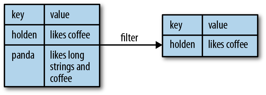
Figure 4-1. Filter on value
Sometimes working with pairs can be awkward if we want to access only the value part of our pair RDD.
Since this is a common pattern, Spark provides the mapValues(func) function, which is the same as map{case (x, y): (x, func(y))}. We will use this function in many of our examples.
We now discuss each of the families of pair RDD functions, starting with aggregations.
Aggregations
When datasets are described in terms of key/value pairs, it is common to want to aggregate statistics across all elements with the same key. We have looked at the fold(), combine(), and reduce() actions on basic RDDs, and similar per-key transformations exist on pair RDDs. Spark has a similar set of operations that combines values that have the same key. These operations return RDDs and thus are transformations rather than actions.
reduceByKey() is quite similar to reduce(); both take a function and use it to combine values.
reduceByKey() runs several parallel reduce operations, one for each key in the dataset, where each operation combines values that have the same key.
Because datasets can have very large numbers of keys, reduceByKey() is not implemented as an action that returns a value to the user program.
Instead, it returns a new RDD consisting of each key and the reduced value for that key.
foldByKey() is quite similar to fold(); both use a zero value of the same type of the data in our RDD and combination function. As with fold(), the provided zero value for foldByKey() should have no impact when added with your combination function to another element.
As Examples 4-7 and 4-8 demonstrate, we can use reduceByKey() along with mapValues() to compute the per-key average in a very similar manner to how fold() and map() can be used to compute the entire RDD average (see Figure 4-2).
As with averaging, we can achieve the same result using a more specialized function, which we will cover next.
Example 4-7. Per-key average with reduceByKey() and mapValues() in Python
rdd.mapValues(lambdax:(x,1)).reduceByKey(lambdax,y:(x[0]+y[0],x[1]+y[1]))
Example 4-8. Per-key average with reduceByKey() and mapValues() in Scala
rdd.mapValues(x=>(x,1)).reduceByKey((x,y)=>(x._1+y._1,x._2+y._2))
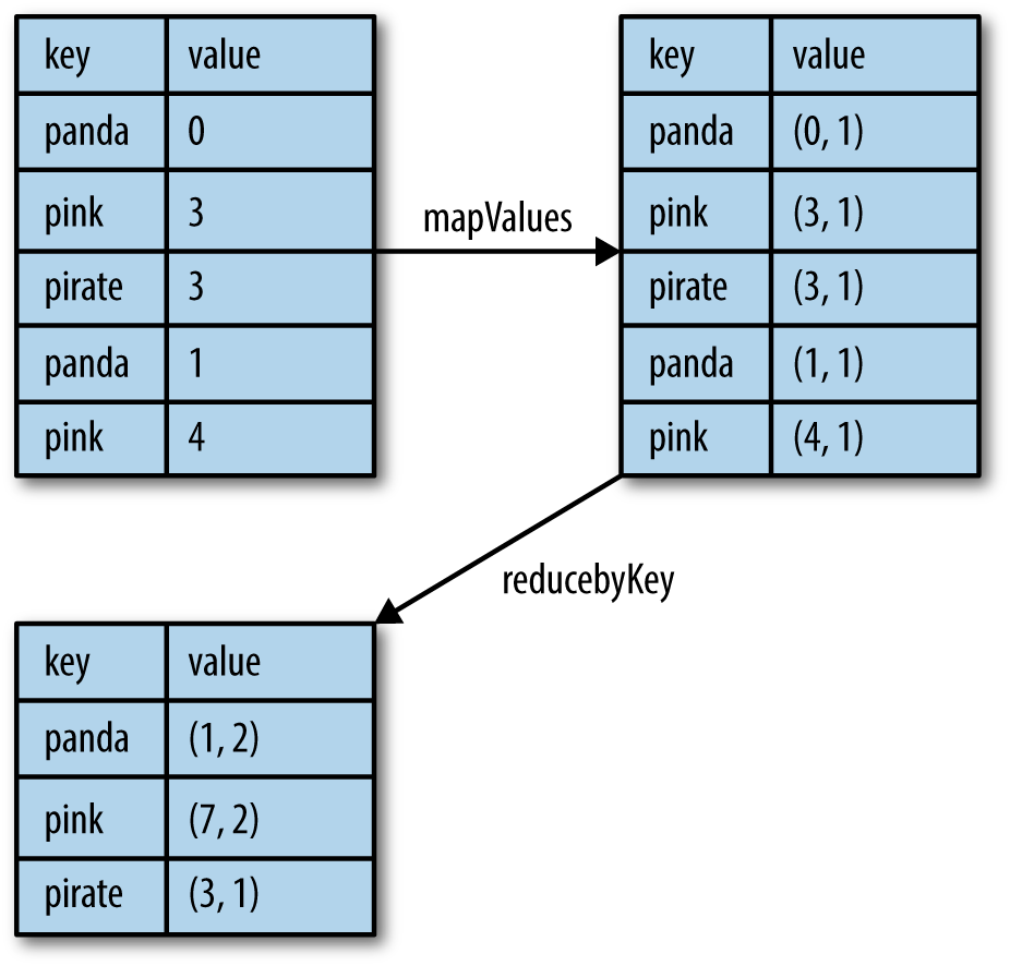
Figure 4-2. Per-key average data flow
Tip
Those familiar with the combiner concept from MapReduce should note that calling reduceByKey() and foldByKey() will automatically perform combining locally on each machine before computing global totals for each key. The user does not need to specify a combiner. The more general combineByKey() interface allows you to customize combining behavior.
We can use a similar approach in Examples 4-9 through 4-11 to also implement the classic distributed word count problem. We will use flatMap() from the previous chapter so that we can produce a pair RDD of words and the number 1 and then sum together all of the words using reduceByKey() as in Examples 4-7 and 4-8.
Example 4-9. Word count in Python
rdd=sc.textFile("s3://...")words=rdd.flatMap(lambdax:x.split(" "))result=words.map(lambdax:(x,1)).reduceByKey(lambdax,y:x+y)
Example 4-10. Word count in Scala
valinput=sc.textFile("s3://...")valwords=input.flatMap(x=>x.split(" "))valresult=words.map(x=>(x,1)).reduceByKey((x,y)=>x+y)
Example 4-11. Word count in Java
JavaRDD<String>input=sc.textFile("s3://...")JavaRDD<String>words=rdd.flatMap(newFlatMapFunction<String,String>(){publicIterable<String>call(Stringx){returnArrays.asList(x.split(" "));}});JavaPairRDD<String,Integer>result=words.mapToPair(newPairFunction<String,String,Integer>(){publicTuple2<String,Integer>call(Stringx){returnnewTuple2(x,1);}}).reduceByKey(newFunction2<Integer,Integer,Integer>(){publicIntegercall(Integera,Integerb){returna+b;}});
Tip
We can actually implement word count even faster by using the countByValue() function on the first RDD: input.flatMap(x => x.split(" ")).countByValue().
combineByKey() is the most general of the per-key aggregation functions.
Most of the other per-key combiners are implemented using it.
Like aggregate(), combineByKey() allows the user to return values that are not the same type as our input data.
To understand combineByKey(), it’s useful to think of how it handles each element it processes. As combineByKey() goes through the elements in a partition, each element either has a key it hasn’t seen before or has the same key as a previous element.
If it’s a new element, combineByKey() uses a function we provide, called createCombiner(), to create the initial value for the accumulator on that key. It’s important to note that this happens the first time a key is found in each partition, rather than only the first time the key is found in the RDD.
If it is a value we have seen before while processing that partition, it will instead use the provided function, mergeValue(), with the current value for the accumulator for that key and the new value.
Since each partition is processed independently, we can have multiple accumulators for the same key.
When we are merging the results from each partition, if two or more partitions have an accumulator for the same key we merge the
accumulators using the user-supplied mergeCombiners() function.
Tip
We can disable map-side aggregation in combineByKey() if we know that our data won’t benefit from it. For example, groupByKey() disables map-side aggregation as the aggregation function (appending to a list) does not save any space. If we want to disable map-side combines, we need to specify the partitioner; for now you can just use the partitioner on the source RDD by passing rdd.partitioner.
Since combineByKey() has a lot of different parameters it is a great candidate for an explanatory example. To better illustrate how combineByKey() works, we will look at computing the average value for each key, as shown in Examples 4-12 through 4-14 and illustrated in Figure 4-3.
Example 4-12. Per-key average using combineByKey() in Python
sumCount=nums.combineByKey((lambdax:(x,1)),(lambdax,y:(x[0]+y,x[1]+1)),(lambdax,y:(x[0]+y[0],x[1]+y[1])))sumCount.map(lambdakey,xy:(key,xy[0]/xy[1])).collectAsMap()
Example 4-13. Per-key average using combineByKey() in Scala
valresult=input.combineByKey((v)=>(v,1),(acc:(Int,Int),v)=>(acc._1+v,acc._2+1),(acc1:(Int,Int),acc2:(Int,Int))=>(acc1._1+acc2._1,acc1._2+acc2._2)).map{case(key,value)=>(key,value._1/value._2.toFloat)}result.collectAsMap().map(println(_))
Example 4-14. Per-key average using combineByKey() in Java
publicstaticclassAvgCountimplementsSerializable{publicAvgCount(inttotal,intnum){total_=total;num_=num;}publicinttotal_;publicintnum_;publicfloatavg(){returntotal_/(float)num_;}}Function<Integer,AvgCount>createAcc=newFunction<Integer,AvgCount>(){publicAvgCountcall(Integerx){returnnewAvgCount(x,1);}};Function2<AvgCount,Integer,AvgCount>addAndCount=newFunction2<AvgCount,Integer,AvgCount>(){publicAvgCountcall(AvgCounta,Integerx){a.total_+=x;a.num_+=1;returna;}};Function2<AvgCount,AvgCount,AvgCount>combine=newFunction2<AvgCount,AvgCount,AvgCount>(){publicAvgCountcall(AvgCounta,AvgCountb){a.total_+=b.total_;a.num_+=b.num_;returna;}};AvgCountinitial=newAvgCount(0,0);JavaPairRDD<String,AvgCount>avgCounts=nums.combineByKey(createAcc,addAndCount,combine);Map<String,AvgCount>countMap=avgCounts.collectAsMap();for(Entry<String,AvgCount>entry:countMap.entrySet()){System.out.println(entry.getKey()+":"+entry.getValue().avg());}
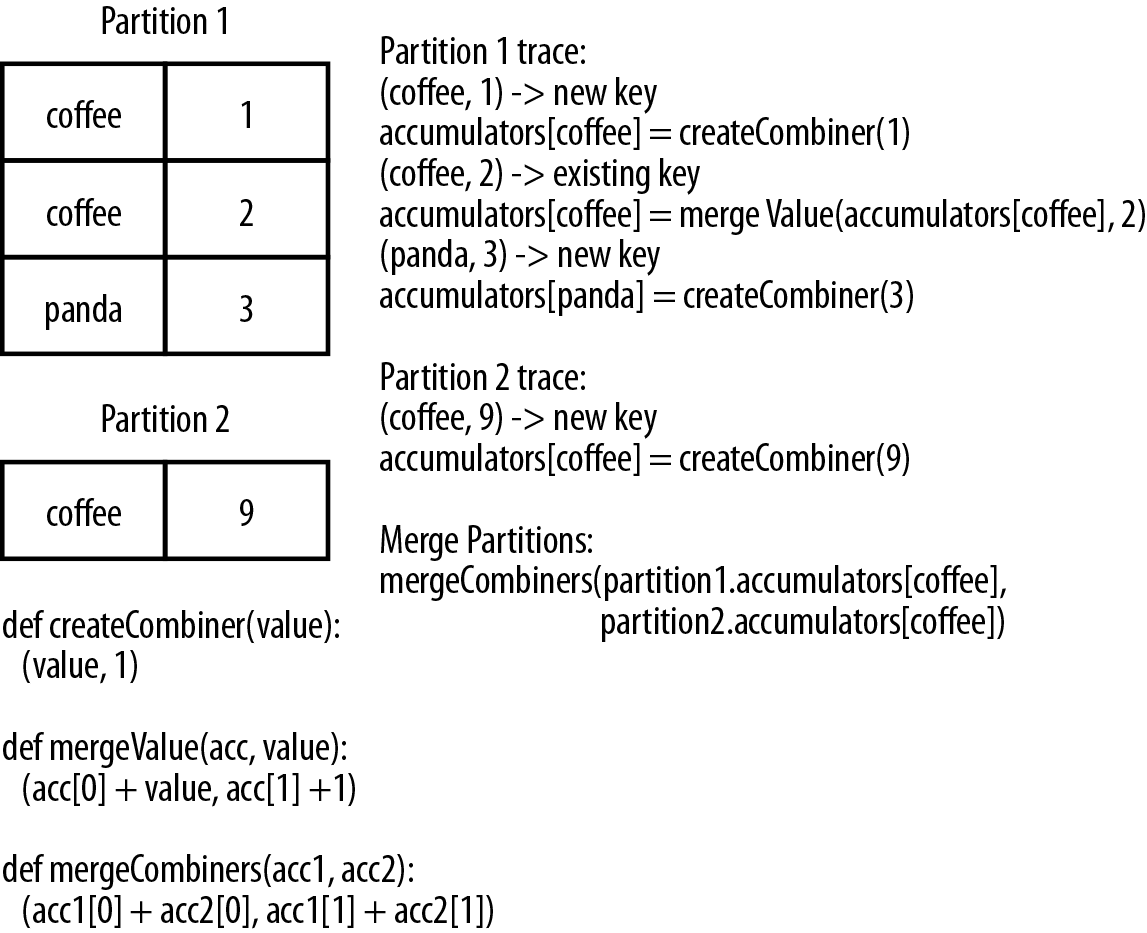
Figure 4-3. combineByKey() sample data flow
There are many options for combining our data by key. Most of them are implemented on top of combineByKey() but provide a simpler interface. In any case, using one of the specialized aggregation functions in Spark can be much faster than the naive approach of grouping our data and then reducing it.
Tuning the level of parallelism
So far we have talked about how all of our transformations are distributed, but we have not really looked at how Spark decides how to split up the work. Every RDD has a fixed number of partitions that determine the degree of parallelism to use when executing operations on the RDD.
When performing aggregations or grouping operations, we can ask Spark to use a specific number of partitions. Spark will always try to infer a sensible default value based on the size of your cluster, but in some cases you will want to tune the level of parallelism for better performance.
Most of the operators discussed in this chapter accept a second parameter giving the number of partitions to use when creating the grouped or aggregated RDD, as shown in Examples 4-15 and 4-16.
Example 4-15. reduceByKey() with custom parallelism in Python
data=[("a",3),("b",4),("a",1)]sc.parallelize(data).reduceByKey(lambdax,y:x+y)# Default parallelismsc.parallelize(data).reduceByKey(lambdax,y:x+y,10)# Custom parallelism
Example 4-16. reduceByKey() with custom parallelism in Scala
valdata=Seq(("a",3),("b",4),("a",1))sc.parallelize(data).reduceByKey((x,y)=>x+y)// Default parallelismsc.parallelize(data).reduceByKey((x,y)=>x+y)// Custom parallelism
Sometimes, we want to change the partitioning of an RDD outside the context of grouping and aggregation operations. For those cases, Spark provides the repartition() function, which shuffles the data across the network to create a new set of partitions.
Keep in mind that repartitioning your data is a fairly expensive operation.
Spark also has an optimized version of repartition() called coalesce() that allows avoiding data movement, but only if you are decreasing the number of RDD partitions.
To know whether you can safely call coalesce(), you can check the size of the RDD using rdd.partitions.size() in Java/Scala and rdd.getNumPartitions() in Python and make sure that you are coalescing it to fewer partitions than it currently has.
Grouping Data
With keyed data a common use case is grouping our data by key—for example, viewing all of a customer’s orders together.
If our data is already keyed in the way we want, groupByKey() will group our data using the key in our RDD. On an RDD consisting of keys of type K and values of type V, we get back an RDD of type [K, Iterable[V]].
groupBy() works on unpaired data or data where we want to use a different condition besides equality on the current key. It takes a function that it applies to every element in the source RDD and uses the result to determine the key.
Tip
If you find yourself writing code where you groupByKey() and then use a reduce() or fold() on the values, you can probably achieve the same result more efficiently by using one of the per-key aggregation functions. Rather than reducing the RDD to an in-memory value, we reduce the data per key and get back an RDD with the reduced values corresponding to each key. For example, rdd.reduceByKey(func) produces the same RDD as rdd.groupByKey().mapValues(value => value.reduce(func)) but is more efficient as it avoids the step of creating a list of values for each key.
In addition to grouping data from a single RDD, we can group data sharing the same key from multiple RDDs using a function called cogroup(). cogroup() over two RDDs sharing the same key type, K, with the respective value types V and W gives us back RDD[(K, (Iterable[V], Iterable[W]))]. If one of the RDDs doesn’t have elements for a given key that is present in the other RDD, the corresponding Iterable is simply empty. cogroup() gives us the power to group data from multiple RDDs.
cogroup() is used as a building block for the joins we discuss in the next section.
Tip
cogroup() can be used for much more than just implementing joins.
We can also use it to implement intersect by key.
Additionally, cogroup() can work on three or more RDDs at once.
Joins
Some of the most useful operations we get with keyed data comes from using it together with other keyed data. Joining data together is probably one of the most common operations on a pair RDD, and we have a full range of options including right and left outer joins, cross joins, and inner joins.
The simple join operator is an inner join.3 Only keys that are present in both pair RDDs are output. When there are multiple values for the same key in one of the inputs, the resulting pair RDD will have an entry for every possible pair of values with that key from the two input RDDs. A simple way to understand this is by looking at Example 4-17.
Example 4-17. Scala shell inner join
storeAddress={(Store("Ritual"),"1026 Valencia St"),(Store("Philz"),"748 Van Ness Ave"),(Store("Philz"),"3101 24th St"),(Store("Starbucks"),"Seattle")}storeRating={(Store("Ritual"),4.9),(Store("Philz"),4.8))}storeAddress.join(storeRating)=={(Store("Ritual"),("1026 Valencia St",4.9)),(Store("Philz"),("748 Van Ness Ave",4.8)),(Store("Philz"),("3101 24th St",4.8))}
Sometimes we don’t need the key to be present in both RDDs to want it in our result. For example, if we were joining customer information with recommendations we might not want to drop customers if there were not any recommendations yet. leftOuterJoin(other) and rightOuterJoin(other) both join pair RDDs together by key, where one of the pair RDDs can be missing the key.
With leftOuterJoin() the resulting pair RDD has entries for each key in the source RDD. The value associated with each key in the result is a tuple of the value from the source RDD and an Option (or Optional in Java) for the value from the other pair RDD. In Python, if a value isn’t present None is used; and if the value is present the regular value, without any wrapper, is used. As with join(), we can have multiple entries for each key; when this occurs, we get the Cartesian product between the two lists of values.
Tip
Optional is part of Google’s Guava library and represents a possibly missing value. We can check isPresent() to see if it’s set, and get() will return the contained instance provided data is present.
rightOuterJoin() is almost identical to leftOuterJoin() except the key must be present in the other RDD and the tuple has an option for the source rather than the other RDD.
We can revisit Example 4-17 and do a leftOuterJoin() and a rightOuterJoin() between the two pair RDDs we used to illustrate join() in Example 4-18.
Example 4-18. leftOuterJoin() and rightOuterJoin()
storeAddress.leftOuterJoin(storeRating)=={(Store("Ritual"),("1026 Valencia St",Some(4.9))),(Store("Starbucks"),("Seattle",None)),(Store("Philz"),("748 Van Ness Ave",Some(4.8))),(Store("Philz"),("3101 24th St",Some(4.8)))}storeAddress.rightOuterJoin(storeRating)=={(Store("Ritual"),(Some("1026 Valencia St"),4.9)),(Store("Philz"),(Some("748 Van Ness Ave"),4.8)),(Store("Philz"),(Some("3101 24th St"),4.8))}
Sorting Data
Having sorted data is quite useful in many cases, especially when you’re producing downstream output. We can sort an RDD with key/value pairs provided that there is an ordering defined on the key.
Once we have sorted our data, any subsequent call on the sorted data to collect() or save() will result in ordered data.
Since we often want our RDDs in the reverse order, the sortByKey() function takes a parameter called ascending indicating whether we want it in ascending order (it defaults to true). Sometimes we want a different sort order entirely, and to support this we can provide our own comparison function. In Examples 4-19 through 4-21, we will sort our RDD by converting the integers to strings and using the string comparison functions.
Example 4-19. Custom sort order in Python, sorting integers as if strings
rdd.sortByKey(ascending=True,numPartitions=None,keyfunc=lambdax:str(x))
Example 4-20. Custom sort order in Scala, sorting integers as if strings
valinput:RDD[(Int,Venue)]=...implicitvalsortIntegersByString=newOrdering[Int]{overridedefcompare(a:Int,b:Int)=a.toString.compare(b.toString)}rdd.sortByKey()
Example 4-21. Custom sort order in Java, sorting integers as if strings
classIntegerComparatorimplementsComparator<Integer>{publicintcompare(Integera,Integerb){returnString.valueOf(a).compareTo(String.valueOf(b))}}rdd.sortByKey(comp)
Actions Available on Pair RDDs
As with the transformations, all of the traditional actions available on the base RDD are also available on pair RDDs. Some additional actions are available on pair RDDs to take advantage of the key/value nature of the data; these are listed in Table 4-3.
| Function | Description | Example | Result |
|---|---|---|---|
|
|
|
|
|
|
|
|
|
|
|
There are also multiple other actions on pair RDDs that save the RDD, which we will describe in Chapter 5.
Data Partitioning (Advanced)
The final Spark feature we will discuss in this chapter is how to control datasets’ partitioning across nodes. In a distributed program, communication is very expensive, so laying out data to minimize network traffic can greatly improve performance. Much like how a single-node program needs to choose the right data structure for a collection of records, Spark programs can choose to control their RDDs’ partitioning to reduce communication. Partitioning will not be helpful in all applications—for example, if a given RDD is scanned only once, there is no point in partitioning it in advance. It is useful only when a dataset is reused multiple times in key-oriented operations such as joins. We will give some examples shortly.
Spark’s partitioning is available on all RDDs of key/value pairs, and causes the system to group elements based on a function of each key. Although Spark does not give explicit control of which worker node each key goes to (partly because the system is designed to work even if specific nodes fail), it lets the program ensure that a set of keys will appear together on some node. For example, you might choose to hash-partition an RDD into 100 partitions so that keys that have the same hash value modulo 100 appear on the same node. Or you might range-partition the RDD into sorted ranges of keys so that elements with keys in the same range appear on the same node.
As a simple example, consider an application that keeps a large table of user information
in memory—say, an RDD of (UserID, UserInfo) pairs, where UserInfo contains a list of
topics the user is subscribed to. The application periodically combines this table with a smaller
file representing events that happened in the past five minutes—say, a table of
(UserID, LinkInfo) pairs for users who have clicked a link on a website in those five
minutes. For example, we may wish to count how many users visited a link that was not to
one of their subscribed topics. We can perform this combination with Spark’s join() operation,
which can be used to group the UserInfo and LinkInfo pairs for each UserID by key.
Our application would look like Example 4-22.
Example 4-22. Scala simple application
// Initialization code; we load the user info from a Hadoop SequenceFile on HDFS.// This distributes elements of userData by the HDFS block where they are found,// and doesn't provide Spark with any way of knowing in which partition a// particular UserID is located.valsc=newSparkContext(...)valuserData=sc.sequenceFile[UserID,UserInfo]("hdfs://...").persist()// Function called periodically to process a logfile of events in the past 5 minutes;// we assume that this is a SequenceFile containing (UserID, LinkInfo) pairs.defprocessNewLogs(logFileName:String){valevents=sc.sequenceFile[UserID,LinkInfo](logFileName)valjoined=userData.join(events)// RDD of (UserID, (UserInfo, LinkInfo)) pairsvaloffTopicVisits=joined.filter{case(userId,(userInfo,linkInfo))=>// Expand the tuple into its components!userInfo.topics.contains(linkInfo.topic)}.count()println("Number of visits to non-subscribed topics: "+offTopicVisits)}
This code will run fine as is, but it will be inefficient. This is because the join() operation,
called each time processNewLogs() is invoked, does not know anything about how the keys are partitioned
in the datasets. By default, this operation will hash all the keys of both datasets, sending elements with the
same key hash across the network to the same machine, and then join together the elements with the same key on that machine (see Figure 4-4). Because we expect the userData table to be much larger than the
small log of events seen every five minutes, this wastes a lot of work: the userData table
is hashed and shuffled across the network on every call, even though it doesn’t change.
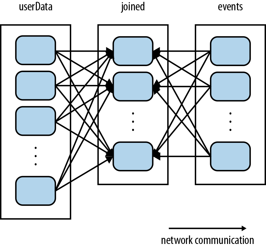
Figure 4-4. Each join of userData and events without using partitionBy()
Fixing this is simple: just use the partitionBy() transformation on userData to hash-partition
it at the start of the program. We do this by passing a spark.HashPartitioner object to
partitionBy, as shown in Example 4-23.
Example 4-23. Scala custom partitioner
valsc=newSparkContext(...)valuserData=sc.sequenceFile[UserID,UserInfo]("hdfs://...").partitionBy(newHashPartitioner(100))// Create 100 partitions.persist()
The processNewLogs() method can remain unchanged: the events RDD is local to processNewLogs(),
and is used only once within this method, so there is no advantage in specifying a partitioner for
events. Because we called partitionBy() when building
userData, Spark will now know that it is hash-partitioned, and calls to join() on it will
take advantage of this information. In particular, when we call userData.join(events), Spark will
shuffle only the events RDD, sending events with each particular UserID to the machine that
contains the corresponding hash partition of userData (see Figure 4-5). The result is that a lot less data is
communicated over the network, and the program runs significantly faster.
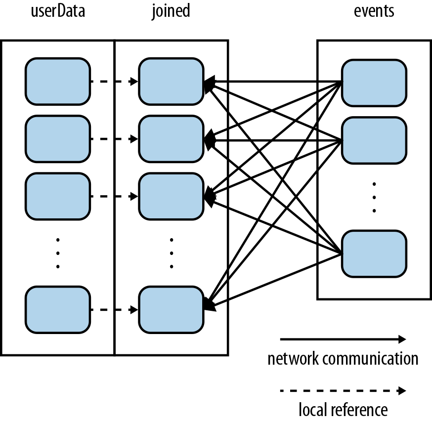
Figure 4-5. Each join of userData and events using partitionBy()
Note that partitionBy() is a transformation, so it always returns a new RDD—it does not
change the original RDD in place. RDDs can never be modified once created. Therefore it is
important to persist and save as userData the result of partitionBy(), not the original
sequenceFile(). Also, the 100 passed to partitionBy() represents the number of partitions,
which will control how many parallel tasks perform further operations on the RDD (e.g., joins);
in general, make this at least as large as the number of cores in your cluster.
Warning
Failure to persist an RDD after it has been transformed with partitionBy() will cause
subsequent uses of the RDD to repeat the partitioning of the data. Without persistence, use of
the partitioned RDD will cause reevaluation of the RDDs complete lineage. That would negate
the advantage of partitionBy(), resulting in repeated partitioning and shuffling of data across
the network, similar to what occurs without any specified partitioner.
In fact, many other Spark operations automatically result in an RDD with known partitioning information,
and many operations other than join() will take advantage of this information. For example, sortByKey()
and groupByKey() will result in range-partitioned and hash-partitioned RDDs, respectively.
On the other hand, operations like map() cause the new RDD to forget the parent’s partitioning
information, because such operations could theoretically modify the key of each record. The next few sections
describe how to determine how an RDD is partitioned, and exactly how partitioning affects the
various Spark operations.
Partitioning in Java and Python
Spark’s Java and Python APIs benefit from partitioning in the same way as the Scala API. However,
in Python, you cannot pass a HashPartitioner object to partitionBy; instead, you just pass
the number of partitions desired (e.g., rdd.partitionBy(100)).
Determining an RDD’s Partitioner
In Scala and Java, you can determine how an RDD is partitioned using its partitioner property
(or partitioner() method in Java).4
This returns a scala.Option object, which is a Scala class
for a container that may or may not contain one item.
You can call isDefined() on the Option to check whether it has a value, and get() to get
this value. If present, the value will be a spark.Partitioner object. This is essentially
a function telling the RDD which partition each key goes into; we’ll talk more about this later.
The partitioner property is a great way to test in the Spark shell how different Spark operations affect
partitioning, and to check that the operations you want to do in your program
will yield the right result (see Example 4-24).
Example 4-24. Determining partitioner of an RDD
scala>valpairs=sc.parallelize(List((1,1),(2,2),(3,3)))pairs:spark.RDD[(Int,Int)]=ParallelCollectionRDD[0]atparallelizeat<console>:12scala>pairs.partitionerres0:Option[spark.Partitioner]=Nonescala>valpartitioned=pairs.partitionBy(newspark.HashPartitioner(2))partitioned:spark.RDD[(Int,Int)]=ShuffledRDD[1]atpartitionByat<console>:14scala>partitioned.partitionerres1:Option[spark.Partitioner]=Some(spark.HashPartitioner@5147788d)
In this short session, we created an RDD of (Int, Int) pairs, which initially have no
partitioning information (an Option with value None). We then created a second RDD by
hash-partitioning the first. If we actually wanted to use partitioned in further
operations, then we should have appended persist() to the third line of input, in which partitioned
is defined. This is for the same reason that we needed persist() for userData in the previous
example: without persist(), subsequent RDD actions will evaluate the entire lineage of
partitioned, which will cause pairs to be hash-partitioned over and over.
Operations That Benefit from Partitioning
Many of Spark’s operations involve shuffling data by key across the network. All of these will
benefit from partitioning. As of Spark 1.0, the operations that benefit from partitioning are
cogroup(),
groupWith(),
join(),
leftOuterJoin(),
rightOuterJoin(),
groupByKey(),
reduceByKey(),
combineByKey(), and
lookup().
For operations that act on a single RDD, such as reduceByKey(), running on a pre-partitioned
RDD will cause all the values for each key to be computed locally on a single machine,
requiring only the final, locally reduced value to be sent from each worker node back to the master. For binary operations, such
as cogroup() and join(), pre-partitioning will cause at least one of the RDDs (the one with the known
partitioner) to not be shuffled. If both RDDs have the same partitioner, and if they are
cached on the same machines (e.g., one was created using mapValues() on the other, which preserves
keys and partitioning) or if one
of them has not yet been computed, then no shuffling across the network will occur.
Operations That Affect Partitioning
Spark knows internally how each of its operations affects partitioning, and automatically
sets the partitioner on RDDs created by operations that partition the data. For example,
suppose you called join() to join two RDDs; because the elements with the same key have
been hashed to the same machine, Spark knows that the result is hash-partitioned, and
operations like reduceByKey() on the join result are going to be significantly faster.
The flipside, however, is that for transformations that cannot be guaranteed to produce a
known partitioning, the output RDD will not have a partitioner set. For example, if you
call map() on a hash-partitioned RDD of key/value pairs, the function passed to map() can
in theory change the key of each element, so the result will not have a partitioner. Spark
does not analyze your functions to check whether they retain the key. Instead, it provides
two other operations, mapValues() and flatMapValues(), which guarantee that each tuple’s
key remains the same.
All that said, here are all the operations that result in a partitioner being set on the
output RDD:
cogroup(),
groupWith(),
join(),
leftOuterJoin(),
rightOuterJoin(),
groupByKey(),
reduceByKey(),
combineByKey(),
partitionBy(),
sort(),
mapValues() (if the parent RDD has a partitioner),
flatMapValues() (if parent has a partitioner), and
filter() (if parent has a partitioner).
All other operations will produce a result with no partitioner.
Finally, for binary operations, which partitioner is set on the output depends on the parent RDDs’ partitioners.
By default, it is a hash partitioner, with the number of partitions set to the level of
parallelism of the operation. However, if one of the parents has a partitioner set,
it will be that partitioner; and if both parents have a partitioner set, it will be the
partitioner of the first parent.
Example: PageRank
As an example of a more involved algorithm that can benefit from RDD partitioning, we consider PageRank. The PageRank algorithm, named after Google’s Larry Page, aims to assign a measure of importance (a “rank”) to each document in a set based on how many documents have links to it. It can be used to rank web pages, of course, but also scientific articles, or influential users in a social network.
PageRank is an iterative algorithm that performs many joins, so it is a good use case for RDD
partitioning. The algorithm maintains two datasets: one of (pageID, linkList) elements
containing the list of neighbors of each page, and one of (pageID, rank) elements containing
the current rank for each page. It proceeds as follows:
-
Initialize each page’s rank to 1.0.
-
On each iteration, have page
psend a contribution ofrank(p)/numNeighbors(p)to its neighbors (the pages it has links to). -
Set each page’s rank to
0.15 + 0.85 * contributionsReceived.
The last two steps repeat for several iterations, during which the algorithm will converge to the correct PageRank value for each page. In practice, it’s typical to run about 10 iterations.
Example 4-25 gives the code to implement PageRank in Spark.
Example 4-25. Scala PageRank
// Assume that our neighbor list was saved as a Spark objectFilevallinks=sc.objectFile[(String,Seq[String])]("links").partitionBy(newHashPartitioner(100)).persist()// Initialize each page's rank to 1.0; since we use mapValues, the resulting RDD// will have the same partitioner as linksvarranks=links.mapValues(v=>1.0)// Run 10 iterations of PageRankfor(i<-0until10){valcontributions=links.join(ranks).flatMap{case(pageId,(links,rank))=>links.map(dest=>(dest,rank/links.size))}ranks=contributions.reduceByKey((x,y)=>x+y).mapValues(v=>0.15+0.85*v)}// Write out the final ranksranks.saveAsTextFile("ranks")
That’s it! The algorithm starts with a ranks RDD initialized at 1.0 for each element, and
keeps updating the ranks variable on each iteration. The body of PageRank is pretty simple to
express in Spark: it first does a join() between the current ranks RDD and the static links
one, in order to obtain the link list and rank for each page ID together, then uses this in a
flatMap to create “contribution” values to send to each of the page’s neighbors. We then
add up these values by page ID (i.e., by the page receiving the contribution) and set that page’s
rank to 0.15 + 0.85 * contributionsReceived.
Although the code itself is simple, the example does several things to ensure that the RDDs are partitioned in an efficient way, and to minimize communication:
-
Notice that the
linksRDD is joined againstrankson each iteration. Sincelinksis a static dataset, we partition it at the start withpartitionBy(), so that it does not need to be shuffled across the network. In practice, thelinksRDD is also likely to be much larger in terms of bytes thanranks, since it contains a list of neighbors for each page ID instead of just aDouble, so this optimization saves considerable network traffic over a simple implementation of PageRank (e.g., in plain MapReduce). -
For the same reason, we call
persist()onlinksto keep it in RAM across iterations. -
When we first create
ranks, we usemapValues()instead ofmap()to preserve the partitioning of the parent RDD (links), so that our first join against it is cheap. -
In the loop body, we follow our
reduceByKey()withmapValues(); because the result ofreduceByKey()is already hash-partitioned, this will make it more efficient to join the mapped result againstlinkson the next iteration.
Tip
To maximize the potential for partitioning-related optimizations, you should use mapValues() or
flatMapValues() whenever you are not changing an element’s key.
Custom Partitioners
While Spark’s HashPartitioner and RangePartitioner are well suited to many use cases, Spark also allows you to tune
how an RDD is partitioned by providing a custom Partitioner object. This can help you further
reduce communication by taking advantage of domain-specific knowledge.
For example, suppose we wanted to run the PageRank algorithm in the previous section on a set of
web pages. Here each page’s ID (the key in our RDD) will be its URL. Using a simple hash function
to do the partitioning, pages with similar URLs (e.g., http://www.cnn.com/WORLD and
http://www.cnn.com/US) might be hashed to completely different nodes. However, we know that web
pages within the same domain tend to link to each other a lot. Because PageRank needs to send a
message from each page to each of its neighbors on each iteration, it helps to group these pages
into the same partition. We can do this with a custom Partitioner that looks at just the domain
name instead of the whole URL.
To implement a custom partitioner, you need to subclass the org.apache.spark.Partitioner class and
implement three methods:
-
numPartitions: Int, which returns the number of partitions you will create. -
getPartition(key: Any): Int, which returns the partition ID (0 tonumPartitions-1) for a given key. -
equals(), the standard Java equality method. This is important to implement because Spark will need to test yourPartitionerobject against other instances of itself when it decides whether two of your RDDs are partitioned the same way!
One gotcha is that if you rely on Java’s hashCode() method in your algorithm, it can return negative
numbers. You need to be careful to ensure that getPartition() always returns a nonnegative result.
Example 4-26 shows how we would write the domain-name-based partitioner sketched previously, which hashes only the domain name of each URL.
Example 4-26. Scala custom partitioner
classDomainNamePartitioner(numParts:Int)extendsPartitioner{overridedefnumPartitions:Int=numPartsoverridedefgetPartition(key:Any):Int={valdomain=newJava.net.URL(key.toString).getHost()valcode=(domain.hashCode%numPartitions)if(code<0){code+numPartitions// Make it non-negative}else{code}}// Java equals method to let Spark compare our Partitioner objectsoverridedefequals(other:Any):Boolean=othermatch{casednp:DomainNamePartitioner=>dnp.numPartitions==numPartitionscase_=>false}}
Note that in the equals() method, we used Scala’s pattern matching operator (match) to
test whether other is a DomainNamePartitioner, and cast it if so; this is the same as
using instanceof() in Java.
Using a custom Partitioner is easy: just pass it to the partitionBy() method. Many of the
shuffle-based methods in Spark, such as join() and groupByKey(), can also take an optional
Partitioner object to control the partitioning of the output.
Creating a custom Partitioner in Java is very similar to Scala: just extend the
spark.Partitioner class and implement the required methods.
In Python, you do not extend a Partitioner class, but instead pass a hash function
as an additional argument to RDD.partitionBy(). Example 4-27 demonstrates.
Example 4-27. Python custom partitioner
importurlparsedefhash_domain(url):returnhash(urlparse.urlparse(url).netloc)rdd.partitionBy(20,hash_domain)# Create 20 partitions
Note that the hash function you pass will be compared by identity to that of other RDDs.
If you want to partition multiple RDDs with the same partitioner, pass the same function
object (e.g., a global function) instead of creating a new lambda for each one!
Conclusion
In this chapter, we have seen how to work with key/value data using the specialized functions available in Spark. The techniques from Chapter 3 also still work on our pair RDDs. In the next chapter, we will look at how to load and save data.
Get Learning Spark now with the O’Reilly learning platform.
O’Reilly members experience books, live events, courses curated by job role, and more from O’Reilly and nearly 200 top publishers.

