Performance management remains one of the key system management disciplines performed by systems professionals of all stripes. For instance, as a LAN administrator, you may be responsible for setting up the hardware platform and operating system environment used to run the applications that your company needs to run its business. The performance aspects of this job include monitoring the hardware and software and making configuration changes and tuning adjustments to make things run better. To support capacity planning and budgeting, you may be called upon to provide measurement data to cost-justify hardware expenditures and as input to the capacity planning process that is designed to ensure that adequate resources continue to be available.
In a capacity planning role, you may be responsible for assuring that adequate resources are available over the long term. This may mean monitoring the current growth, factoring in new application projects, and trying to plan the hardware configuration that can supply adequate performance. This inevitably means that you will encounter your company’s budget for new equipment purchases. You will be called upon to explain your recommendations in straightforward, nontechnical language. Perhaps your analysis will show that more hardware is needed to meet the performance objectives or else workers interacting with the system will not be fully productive. This is part of performance management, too.
Our approach to these and other performance management tasks is decidedly empirical. Remember, you cannot manage what you cannot measure. We recommend that you gather data from real systems in operation, analyze it, and make decisions based on that analysis. Those decisions may range from deciding how to configure a workstation running Windows 2000 Professional for optimal performance for a graphics-intensive application, to how to configure multiple Windows 2000 servers to support distributed database or messaging applications. For systems under development, you may need to discuss hardware and software infrastructure alternatives with the programmers responsible for implementing the application. If you get an opportunity to influence the design of an important application under development, try to link decisions about design trade-offs to actual measurements of prototype code running under different conditions of stress. Before setting parameters and making tuning adjustments, review and analyze performance statistics from the system. Afterwards, verify that the changes you made are working by looking at similar measurement data.
Whatever the challenge, your approach should always be analytical. For example, before making a tuning adjustment, analyze the measurement data and develop a working hypothesis as to what the problem is and how to solve it. You will rely on a variety of analytical tools, mainly queuing models and statistical analysis. The analysis generates a working hypothesis, which is then tested against further observations. Does the adjustment you made improve the system’s behavior in the way you expected? That is often convincing evidence that the working hypothesis you adopted was an appropriate one.
The empirical approach we recommend contrasts with something we will call the Rule of Thumb approach. Rules of thumb (ROTs) are received wisdom passed down from professed experts to the masses. This sounds like a great approach since these self-appointed wizards appear to know much more about the sacred innards of Windows 2000 than you do. The problem with these pearls of wisdom is that they may not apply to your specific environment. We think you should find out how these great seers derived the rule being espoused, attempt to apply the same derivation to your environment, and determine for yourself if the rule is applicable. Quite possibly, after you have modified the rule to your specific environment, it may very well be relevant to your situation.
For example, our approach to evaluating whether or not to do a memory upgrade begins with the hypothesis that the amount of paging is related to an index of memory utilization we can calculate. The difference between a Windows 2000 server configured at 256 MB versus one configured at 512 MB might be a significant amount of money. If multiple Windows 2000 servers or workstations are involved, the dollars start to add up fast. The memory utilization index you need to calculate is the number of committed virtual memory bytes divided by the amount of hardware RAM installed. Look to find empirical evidence in the performance measurements that a relationship exists between the memory utilization index and paging activity. If this relationship does exist and you understand its behavior, you may be able to use it to estimate the benefits of a memory upgrade. This particular technique is discussed in greater detail in Chapter 6.
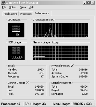
If we know that this relationship exists on many different systems, we might then distill the evidence into a general configuration rule. Without much further analysis, we might suggest that a good configuration rule of thumb is to provide at least 1 MB of RAM for every 2 MB of committed virtual memory. This is a very easy rule to apply because you can simply run the Task Manager application and access the Performance tab to determine the Commit Charge (K) total virtual memory peak (see Figure 1-6). Divide the Commit Charge (K) total by the Physical Memory (K) total field. If that ratio is 2 or more, it may be time to buy more memory for that machine. Remember, however, that your mileage may vary. Rather than just blindly applying this rule, we want you to understand how the rule was derived and be capable of adapting the method to your particular set of circumstances. We will discuss the empirical evidence used to derive this rule in Chapter 6, and try to explain how you can test to see whether this rule will work for you.
Before proceeding further, there is a common notion that needs to be dispelled. This is the belief that performance considerations in the design and development of computer applications no longer matter because computing resources are so inexpensive. Advocates of this position concede that there may be a few instances where performance is still an important consideration today, but if you just wait a couple more years, these problems will be solved as the hardware keeps getting faster and cheaper.
We have heard this claim that “performance doesn’t matter anymore” for at least 10 years, and we do not believe it is any truer today than it was a decade ago. First, though, we should admit that our perspective is warped because we are frequently the “outside expert” who is called in only during a crisis. Most people do not call the fire department until they have a fire. So we tend to see extreme situations where people are desperate for a solution and do not know where else to turn. Amazingly, many of these problems are very easy to diagnose and can often be solved right over the phone. On the other hand, some problems take weeks and months worth of effort to solve. And some of them, we are sorry to say, are never resolved to everyone’s satisfaction. (There is a joke that no one ever said computer science was an exact science.) Seeing only the more extreme cases tends to warp your perspective. However, we do see just as many of these problems today that we did ten years ago, so it does not seem reasonable to believe bigger and better hardware has solved all our performance problems. Computer performance is still a topic worthy of your consideration.
On the other hand, it is certainly true that the strides taken to improve the performance of hardware have been phenomenal. The PC that sits on our desktop today is a splendid piece of equipment. It costs considerably less money than you would have paid for a 640K PC/XT just 15 years ago. It has five hundred times more memory and about thousand times more disk space. It is lightning-fast at most tasks (although it is still painfully slow at others). Yes, hardware is improving rapidly, but it is important to realize that not all hardware advances at the same rate. For example, advances in disk performance have not been as rapid as instruction processing speeds. Moreover, even as the hardware gets cheaper and cheaper, there are always applications that demand even more resources than we have available.
In addition, computer performance continues to have a cost dimension to it that remains very significant. Many aspects of hardware design reflect cost/performance trade-offs, and it’s important to understand what these are. A software developer still needs to understand how algorithms perform and especially how they scale as the problem space becomes larger or more users are added to the system. Finished designs for any nontrivial system are always compromises that aim for the best balance between performance and cost.
To make the best planning decisions, a traditional approach is to try and understand hardware speeds and feeds -- how fast different pieces of equipment are capable of running. This is much more difficult than it sounds. For example, it certainly seems like a SCSI disk attached to a 20 MB/second SCSI-2 adapter card should run much slower than one attached to an 80 MB/second UltraSCSI-3 adapter card. UltraSCSI-3 sounds as if should beat ol’ SCSI-2 every time. But there may be little or no practical difference in the performance of the two configurations. (Perhaps the disk may only transfer data at 20 MB/second anyway, so the extra capacity of the UltraSCSI-3 bus is not being utilized.)
This example illustrates the principle that a complex system will run only as fast as its slowest component. Because there is both theory and extensive empirical data to back up this claim, we don’t mind propagating this statement as a good rule of thumb. In fact, it provides the theoretical underpinning for a very useful analysis technique, which we will call bottleneck analysis. The slowest device in a configuration is often the weakest link. Find it and replace it with a faster component and you have a good chance that performance will improve. Sounds good, but you probably noticed that the rule does not tell you howto find this component. Given the complexity of many modern computer networks, this seemingly simple task is as easy as finding a needle in the proverbial haystack. Of course, replace some component other than the bottleneck device with a faster component and performance will remain the same.
In both theory and practice, performance tuning is the process of locating the bottleneck in a configuration and removing it. The system’s performance will improve until the next bottleneck is manifest, which you again identify and remove. Removing the bottlenecked device usually entails replacing it with a newer, faster version of the same component. For example, if network bandwidth is a constraint on performance, upgrade the configuration from 10 Mb Ethernet to 100 Mb Fast Ethernet. If the network actually is the bottleneck, performance should improve.
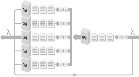
A system in which all bottlenecks have been removed can be said to be a balanced system. All components in a balanced system are at least capable of handling the flow of work from component to component without delays building up at any one particular component. Visualize a network of computing components where work flows from one component (the CPU) to another (the disk), back again, then to another (the network), and back again to the CPU (see Figure 1-7). When different components are evenly distributed across the hardware, that system is balanced. It can even be proved mathematically that performance is optimal when a system is balanced in this fashion.
We can visualize that the balanced system (and not one that is simply over-configured) is one where workload components are evenly distributed across the processing resources. If there are delays, the work that is waiting to be processed is also evenly distributed in the system. This work is illustrated by the shaded areas in Figure 1-8. Suppose we could crank up the rate at which requests arrive to be serviced (think of SQL Server requests to a Windows 2000 database server, for example, or logon requests to an Active Directory authentication server). If the system is balanced, we will observe that work waiting to be processed remains evenly distributed around the system as in Figure 1-8, but there is more of a backlog of requests that need distributing.
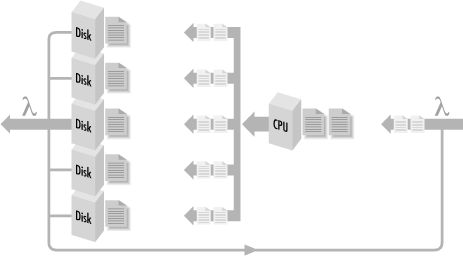
Figure 1-8. A balanced system where shaded areas indicate work queued for processing at different hardware components
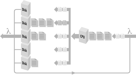
If instead we observe something like Figure 1-9, where many requests are waiting behind just one of the resources, we can then say with some authority that that component isthe bottleneck in the configuration. When work backs up behind a bottlenecked device, delays there may cascade, causing delays elsewhere in the configuration. Because the flow of work through the system is not a simple chain of events, but an interconnected network, the way that the delayed work impacts processing at other components may not always be obvious. Empirically, it is sufficient to observe that work accumulates behind the bottlenecked device at faster rates as the workload increases. Replacing this component with a faster one should improve the rate that work can flow through the entire system. So now you know that “computer performance analyst” is just a fancy term for a computer plumber who goes around clearing stopped-up drains!
Unfortunately for us computer plumbers, it is not always easy to figure out where bottlenecks are or how to relieve them. Consider the nightly backup process that copies new and updated files to tape so that you can restore a user’s environment when a hard disk crashes. Assume that when you first began backing up files on the computers attached to the LAN to the tape drive attached to the backup server, the process took only four hours each night. Over time, because there are more users and more disks, the process takes longer and longer. Soon there are not enough hours during the evening to back up all the files that need to be backed up. What should be done about this situation?
First, you upgrade the tape drive to a newer model that the manufacturer promises is faster and more powerful. But that does not speed up the process. It is time to begin a search for the bottlenecked device. Unfortunately, there are many potential devices to be considered. Perhaps network bandwidth is the problem, and you need to update hubs, routers, and network interface cards. Perhaps the network is adequate (utilization is low and there are few collisions), but the network cards cannot pump data onto the line fast enough. Perhaps the cards are fine, but the networking software is slowing things down by waiting too long before transmitting the next request. (Maybe the TCP window size is not set correctly.) Perhaps the cards and the networking software are fine, but the client CPU is not able to push data out to the card because the internal bus connecting the card to the computer is not fast enough. Perhaps the hard disk where the files reside simply cannot move the data any faster because files are spread all over the disk instead of being located contiguously (i.e., the disk is fragmented). Perhaps this is not a problem that you are going to solve tonight.
Once you find irrefutable evidence of a bottlenecked device, you want to replace it with a faster component. How do we know that one component is actually faster than another? Will it actually be faster when it comes to your workload? Unfortunately, these questions are not easy to answer either. Worse, there is no general agreement or universally accepted standards of comparison among different machines, platforms, and architectures. This is due to the fact that there are so many workload-dependent factors. This leads us inevitably to the topic of building and executing comparative benchmarks.
Benchmarks are repeatableexecution sequences that can be run on different computers at different times to form a basis of comparison. A benchmarking methodology is as follows. Develop a representative workload that can be executed over and over again. Run the workload on System A and again on System B (which is configured differently) and compare the results. Working hypothesis: Since the execution runs are otherwise identical, any time differences should be a function of differences in the operating environments. A benchmark establishes an apples-to-apples comparison between the performance of two or more systems.
Generally, there are two types of benchmark workloads: realand synthetic. Real (or natural) benchmark workloads are created by capturing actual system usage with a tool that is later used to play back the workload at a controlled rate or with more users. Synthetic benchmarks are sample applications or programs that you acquire purely for testing purposes. The fact that these synthetic applications exist and can be purchased off the shelf is particularly useful when the capacity planning exercise is for an application that remains to be built.
The popularity of the benchmark approach, especially the test results reported extensively in consumer-oriented trade publications, should not be confused with its effectiveness in making configuration decisions. Decision-making based on benchmarks results, even with so-called industry-standard benchmarks, almost always generates serious questions about validity and interpretation. One important consideration is determining that the benchmark is relevant to the kind of work you eventually plan to perform. The fact that the benchmark load, in the case of both real or synthetic benchmarks, is representative of actual workloads is difficult to establish in practice, and once established, is subject to change over time. How can you determine that a given benchmark load is representative of your actual workload? Unfortunately, this is not a question with a simple answer.
Another problem is the assumption that the benchmark is repeatable across many different platforms. You are likely to find that benchmark measurements vary greatly in successive runs on the same configuration. Various cache loading effects are notorious in this regard, and cache techniques are in widespread use. (This is an enormously complicated technical topic that we will pursue in Chapter 6 and Chapter 7.) Manufacturers typically provide speed ratings of their equipment running standard benchmark suites in their development labs. When you attempt to measure performance levels in your own environment, inevitably they suffer by comparison. This leads immediately to the question, “What is different about my environment?” Again, not an easy question to answer. In the case of benchmark results published in the trade press, you may not be able to find out enough about the test configuration to ever make an apples-to-apples comparison to your workload.
These additional elements make benchmarking much more complicated in practice than in theory. Assessing the relative performance of two different processor architectures ought to be as simple as running the same benchmark test against each and evaluating the results. It isn’t. Raw processor performance is typically measured by clock speed and the number of clock cycles needed per instruction. This leads to a standard measure of instructions executed per second (IPS) or Instruction Execution Rate (IER). But which instructions? Reduced Instruction Set Computers (RISC) may require three instructions to perform the same logical operation that a Complex Instruction Set Computer (CISC) can perform in one instruction. Both RISC and CISC computers typically also have pipelines and scalar processing facilities that enable them to execute some, but not all, instruction in parallel. Measurements of actual instruction execution rates vary significantly from workload to workload depending on the instruction mix.
By comparison, measurements of disk speed are relatively standardized. Disks are usually measured in terms of head seek time, rotational delay waiting to locate the desired sector while the device spins, and data transfer rates in bytes per second. However, under benchmark testing conditions, actual disk performance is affected by file placement, disk caching strategies, disk fragmentation, and many other considerations. Network access primarily depends on the speed of the wire, but is complicated by processing delays that occur as packets traverse the network of connections between local area and wide area segments. The network protocol in use also determines how many different messages are sent and received and what sorts of acknowledgments are required. In most realistic circumstances, network topology is so unique that only measurements gathered from the actual running system are trustworthy.
Benchmarks are useful, but be careful in interpreting the results (the widely hyped test scores and ratings in articles and advertisements notwithstanding). Remember, for any of the popular, standardized benchmarks in widespread use, there is also a good deal of benchmark engineering going on back at the factory. The engineers that developed the equipment tested it constantly by running standard benchmarks to see if the latest engineering change yielded any improvement. This is standard practice. Vendors need ways to stress test products under development, and they naturally want to be able to advertise that their equipment received a better score than a competitor’s on a well-known benchmark test.
Frequently, engineers will insert optimizations designed to speed up execution running a specific benchmark. The result of this process is equipment that is very good at running standard benchmark workloads, but may not be so good at running yours. There is nothing wrong with this practice, so long as the benchmark is in fact representative of actual workloads. But it does raise issues of interpretation. There is always the possibility that a particular optimization that accounts for a good benchmark score is not especially useful when it comes to your configuration and workload.
The ideal situation is performing empirical testing with the equipment running your workload. But building a realistic and representative benchmark-testing environment of your own is both expensive and time-consuming. Nor can you test all the different varieties and configuration permutations under consideration. Here, analytic techniques are useful for projecting the performance of proposed configurations from actual performance measurements. Understanding what the characteristics of the benchmark workload are and how they compare to your actual workloads is crucial in performing this type of analysis. Workload characterization is an essential first step in the analysis of both real and synthetic workloads.
Get Windows 2000 Performance Guide now with the O’Reilly learning platform.
O’Reilly members experience books, live events, courses curated by job role, and more from O’Reilly and nearly 200 top publishers.

