Chapter 4. Advanced Windowing
Hello again! I hope you enjoyed Chapter 3 as much as I did. Watermarks are a fascinating topic, and Slava knows them better than anyone on the planet. Now that we have a deeper understanding of watermarks under our belts, I’d like to dive into some more advanced topics related to the what, where, when, and how questions.
We first look at processing-time windowing, which is an interesting mix of both where and when, to understand better how it relates to event-time windowing and get a sense for times when it’s actually the right approach to take. We then dive into some more advanced event-time windowing concepts, looking at session windows in detail, and finally making a case for why generalized custom windowing is a useful (and surprisingly straightforward) concept by exploring three different types of custom windows: unaligned fixed windows, per-key fixed windows, and bounded sessions windows.
When/Where: Processing-Time Windows
Processing-time windowing is important for two reasons:
-
For certain use cases, such as usage monitoring (e.g., web service traffic QPS), for which you want to analyze an incoming stream of data as it’s observed, processing-time windowing is absolutely the appropriate approach to take.
-
For use cases for which the time that events happened is important (e.g., analyzing user behavior trends, billing, scoring, etc.), processing-time windowing is absolutely the wrong approach to take, and being able to recognize these cases is critical.
As such, it’s worth gaining a solid understanding of the differences between processing-time windowing and event-time windowing, particularly given the prevalence of processing-time windowing in many streaming systems today.
When working within a model for which windowing as a first-class notion is strictly event-time based, such as the one presented in this book, there are two methods that you can use to achieve processing-time windowing:
- Triggers
-
Ignore event time (i.e., use a global window spanning all of event time) and use triggers to provide snapshots of that window in the processing-time axis.
- Ingress time
-
Assign ingress times as the event times for data as they arrive, and use normal event-time windowing from there on. This is essentially what something like Spark Streaming 1.x does.
Note that the two methods are more or less equivalent, although they differ slightly in the case of multistage pipelines: in the triggers version, a multistage pipeline will slice the processing-time “windows” independently at each stage, so, for example, data in window N for one stage might instead end up in window N–1 or N+1 in the following stage; in the ingress-time version, after a datum is incorporated into window N, it will remain in window N for the duration of the pipeline due to synchronization of progress between stages via watermarks (in the Cloud Dataflow case), microbatch boundaries (in the Spark Streaming case), or whatever other coordinating factor is involved at the engine level.
As I’ve noted to death, the big downside of processing-time windowing is that the contents of the windows change when the observation order of the inputs changes. To drive this point home in a more concrete manner, we’re going to look at these three use cases: event-time windowing, processing-time windowing via triggers, and processing-time windowing via ingress time.
Each will be applied to two different input sets (so six variations total). The two inputs sets will be for the exact same events (i.e., same values, occurring at the same event times), but with different observation orders. The first set will be the observation order we’ve seen all along, colored gray; the second one will have all the values shifted in the processing-time axis as in Figure 4-1, colored purple. You can simply imagine that the purple example is another way reality could have happened if the winds had been blowing in from the east instead of the west (i.e., the underlying set of complex distributed systems had played things out in a slightly different order).
Figure 4-1. Shifting input observation order in processing time, holding values, and event-times constant
Event-Time Windowing
To establish a baseline, let’s first compare fixed windowing in event time with a heuristic watermark over these two observation orderings. We’ll reuse the early/late code from Example 2-7/Figure 2-10 to get the results shown in Figure 4-2. The lefthand side is essentially what we saw before; the righthand side is the results over the second observation order. The important thing to note here is that even though the overall shape of the outputs differs (due to the different orders of observation in processing time), the final results for the four windows remain the same: 14, 18, 4, and 12.
Figure 4-2. Event-time windowing over two different processing-time orderings of the same inputs
Processing-Time Windowing via Triggers
Let’s now compare this to the two processing-time methods just described. First, we’ll try the triggers method. There are three aspects to making processing-time “windowing” work in this manner:
- Windowing
-
We use the global event-time window because we’re essentially emulating processing-time windows with event-time panes.
- Triggering
-
We trigger periodically in the processing-time domain based on the desired size of the processing-time windows.
- Accumulation
-
We use discarding mode to keep the panes independent from one another, thus letting each of them act like an independent processing-time “window.”
The corresponding code looks something like Example 4-1; note that global windowing is the default in Beam, hence there is no specific override of the windowing strategy.
Example 4-1. Processing-time windowing via repeated, discarding panes of a global event-time window
PCollection<KV<Team, Integer>> totals = input
  .apply(Window.triggering(Repeatedly(AlignedDelay(TWO_MINUTES)))
               .discardingFiredPanes())
  .apply(Sum.integersPerKey());
When executed on a streaming runner against our two different orderings of the input data, the results look like Figure 4-3. Here are some interesting notes about this figure:
-
Because we’re emulating processing-time windows via event-time panes, the “windows” are delineated in the processing-time axis, which means their effective width is measured on the y-axis instead of the x-axis.
-
Because processing-time windowing is sensitive to the order that input data are encountered, the results for each of the “windows” differs for each of the two observation orders, even though the events themselves technically happened at the same times in each version. On the left we get 12, 18, 18, whereas on the right we get 7, 36, 5.
Figure 4-3. Processing-time “windowing” via triggers, over two different processing-time orderings of the same inputs
Processing-Time Windowing via Ingress Time
Lastly, let’s look at processing-time windowing achieved by mapping the event times of input data to be their ingress times. Code-wise, there are four aspects worth mentioning here:
- Time-shifting
-
When elements arrive, their event times need to be overwritten with the time of ingress. We can do this in Beam by providing a new
DoFnthat sets the timestamp of the element to the current time via theoutputWithTimestampmethod. - Windowing
-
Return to using standard event-time fixed windowing.
- Triggering
-
Because ingress time affords the ability to calculate a perfect watermark, we can use the default trigger, which in this case implicitly fires exactly once when the watermark passes the end of the window.
- Accumulation mode
-
Because we only ever have one output per window, the accumulation mode is irrelevant.
The actual code might thus look something like that in Example 4-2.
Example 4-2. Processing-time windowing via repeated, discarding panes of a global event-time window
PCollection<String> raw = IO.read().apply(ParDo.of(
  new DoFn<String, String>() {
    public void processElement(ProcessContext c) {
      c.outputWithTimestmap(new Instant());
    }
  });
PCollection<KV<Team, Integer>> input =
  raw.apply(ParDo.of(new ParseFn());
PCollection<KV<Team, Integer>> totals = input
  .apply(Window.info(FixedWindows.of(TWO_MINUTES))
  .apply(Sum.integersPerKey());
Execution on a streaming engine would look like Figure 4-4. As data arrive, their event times are updated to match their ingress times (i.e., the processing times at arrival), resulting in a rightward horizontal shift onto the ideal watermark line. Here are some interesting notes about this figure:
-
As with the other processing-time windowing example, we get different results when the ordering of inputs changes, even though the values and event times for the input stay constant.
-
Unlike the other example, the windows are once again delineated in the event-time domain (and thus along the x-axis). Despite this, they aren’t bonafide event-time windows; we’ve simply mapped processing time onto the event-time domain, erasing the original record of occurrence for each input and replacing it with a new one that instead represents the time the datum was first observed by the pipeline.
-
Despite this, thanks to the watermark, trigger firings still happen at exactly the same time as in the previous processing-time example. Furthermore, the output values produced are identical to that example, as predicted: 12, 18, 18 on the left, and 7, 36, 5 on the right.
-
Because perfect watermarks are possible when using ingress time, the actual watermark matches the ideal watermark, ascending up and to the right with a slope of one.
Figure 4-4. Processing-time windowing via the use of ingress time, over two different processing-time orderings of the same inputs
Although it’s interesting to see the different ways you can implement processing-time windowing, the big takeaway here is the one I’ve been harping on since the first chapter: event-time windowing is order-agnostic, at least in the limit (actual panes along the way might differ until the input becomes complete); processing-time windowing is not. If you care about the times at which your events actually happened, you must use event-time windowing or your results will be meaningless. I will get off my soapbox now.
Where: Session Windows
Enough with processing-time windowing. Let’s now go back to tried-and-true event-time windowing, but now we’re going to look at one of my favorite features: the dynamic, data-driven windows called sessions.
Sessions are a special type of window that captures a period of activity in the data that is terminated by a gap of inactivity. They’re particularly useful in data analysis because they can provide a view of the activities for a specific user over a specific period of time during which they were engaged in some activity. This allows for the correlation of activities within the session, drawing inferences about levels of engagement based on the lengths of the sessions, and so on.
From a windowing perspective, sessions are particularly interesting in two ways:
-
They are an example of a data-driven window: the location and sizes of the windows are a direct consequence of the input data themselves, rather than being based on some predefined pattern within time, as are fixed and sliding windows.
-
They are also an example of an unaligned window; that is, a window that does not apply uniformly across the data, but instead only to a specific subset of the data (e.g., per user). This is in contrast to aligned windows like fixed and sliding windows, which typically apply uniformly across the data.
For some use cases, it’s possible to tag the data within a single session with a common identifier ahead of time (e.g., a video player that emits heartbeat pings with quality-of-service information; for any given viewing, all of the pings can be tagged ahead of time with a single session ID). In this case, sessions are much easier to construct because it’s basically just a form of grouping by key.
However, in the more general case (i.e., where the actual session itself is not known ahead of time), the sessions must be constructed from the locations of the data within time alone. When dealing with out-of-order data, this becomes particularly tricky.
Figure 4-5 shows an example of this, with five independent records grouped together into session windows with a gap timeout of 60 minutes. Each record starts out in a 60-minute window of its own (a proto-session). Merging together overlapping proto-sessions yields the two larger session windows containing three and two records, respectively.
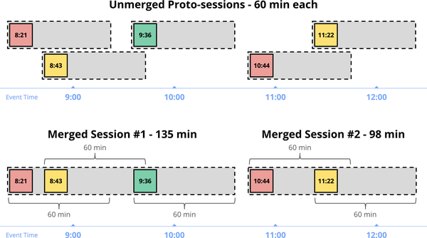
Figure 4-5. Unmerged proto-session windows, and the resultant merged sessions
They key insight in providing general session support is that a complete session window is, by definition, a composition of a set of smaller, overlapping windows, each containing a single record, with each record in the sequence separated from the next by a gap of inactivity no larger than a predefined timeout. Thus, even if we observe the data in the session out of order, we can build up the final session simply by merging together any overlapping windows for individual data as they arrive.
To look at this another way, consider the example we’ve been using so far. If we specify a session timeout of one minute, we would expect to identify two sessions in the data, delineated in Figure 4-6 by the dashed black lines. Each of those sessions captures a burst of activity from the user, with each event in the session separate by less than one minute from at least one other event in the session.
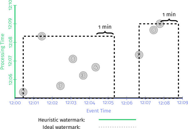
Figure 4-6. Sessions we want to compute
To see how the window merging works to build up these sessions over time as events are encountered, let’s look at it in action. We’ll take the early/late code with retractions enabled from Example 2-10 and update the windowing to build sessions with a one-minute gap duration timeout instead. Example 4-3 illustrates what this looks like.
Example 4-3. Early/on-time/late firings with session windows and retractions
PCollection<KV<Team, Integer>> totals = input
  .apply(Window.into(Sessions.withGapDuration(ONE_MINUTE))
               .triggering(
                 AfterWatermark()
                   .withEarlyFirings(AlignedDelay(ONE_MINUTE))
                   .withLateFirings(AfterCount(1)))
               .accumulatingAndRetractingFiredPanes())
  .apply(Sum.integersPerKey());
Executed on a streaming engine, you’d get something like that shown in Figure 4-7 (note that I’ve left in the dashed black lines annotating the expected final sessions for reference).
Figure 4-7. Early and late firings with session windows and retractions on a streaming engine
There’s quite a lot going on here, so I’ll walk you through some of it:
-
When the first record with value 5 is encountered, it’s placed into a single proto-session window that begins at that record’s event time and spans the width of the session gap duration; for example, one minute beyond the point at which that datum occurred. Any windows we encounter in the future that overlap this window should be part of the same session and will be merged into it as such.
-
The second record to arrive is the 7, which similarly is placed into its own proto-session window, given that it doesn’t overlap with the window for the 5.
-
In the meantime, the watermark has passed the end of the first window, so the value of 5 is materialized as an on-time result just before 12:06. Shortly thereafter, the second window is also materialized as a speculative result with value 7, right as processing time hits 12:06.
-
We next observe a pair of records 3 and 4, the proto-sessions for which overlap. As a result, they are merged together, and by the time the early trigger for 12:07 fires, a single window with value 7 is emitted.
-
When the 8 arrives shortly thereafter, it overlaps with both of the windows with value 7. All three are thus merged together, forming a new combined session with value 22. When the watermark then passes the end of this session, it materializes both the new session with value 22 as well as retractions for the two windows of value 7 that were previously emitted, but later incorporated into it.
-
A similar dance occurs when the 9 arrives late, joining the proto-session with value 5 and session with value 22 into a single larger session of value 36. The 36 and the retractions for the 5 and 22 windows are all emitted immediately by the late data trigger.
This is some pretty powerful stuff. And what’s really awesome is how easy it is to describe something like this within a model that breaks apart the dimensions of stream processing into distinct, composable pieces. In the end, you can focus more on the interesting business logic at hand, and less on the minutiae of shaping the data into some usable form.
If you don’t believe me, check out this blog post describing how to manually build up sessions on Spark Streaming 1.x (note that this is not done to point fingers at them; the Spark folks had just done a good enough job with everything else that someone actually bothered to go to the trouble of documenting what it takes to build a specific variety of sessions support on top of Spark 1.x; you can’t say the same for most other systems out there). It’s quite involved, and they’re not even doing proper event-time sessions, or providing speculative or late firings, or retractions.
Where: Custom Windowing
Up until now, we’ve talked primarily about predefined types of windowing strategies: fixed, sliding, and sessions. You can get a lot of mileage out of standard types of windows, but there are plenty of real-world use cases for which being able to define a custom windowing strategy can really save the day (three of which we’re about to see now).
Most systems today don’t support custom windowing to the degree that it’s supported in Beam,1 so we focus on the Beam approach. In Beam, a custom windowing strategy consists of two things:
- Window assignment
-
This places each element into an initial window. At the limit, this allows every element to be placed within a unique window, which is very powerful.
- (Optional) window merging
-
This allows windows to merge at grouping times, which makes it possible for windows to evolve over time, which we saw in action earlier with session windows.
To give you a sense for how simple windowing strategies really are, and also how useful custom windows support can be, we’re going to look in detail at the stock implementations of fixed windows and sessions in Beam and then consider a few real-world use cases that require custom variations on those themes. In the process, we’ll see both how easy it is to create a custom windowing strategy, and how limiting the lack of custom windowing support can be when your use case doesn’t quite fit into the stock approaches.
Variations on Fixed Windows
To begin, let’s look at the relatively simple strategy of fixed windows. The stock fixed-windows implementation is as straightforward as you might imagine, and consists of the following logic:
- Assignment
-
The element is placed into the appropriate fixed-window based on its timestamp and the window’s size and offset parameters.
- Merging
-
None.
An abbreviated version of the code looks like Example 4-4.
Example 4-4. Abbreviated FixedWindows implementation
publicclassFixedWindowsextendsWindowFn<Object,IntervalWindow>{privatefinalDurationsize;privatefinalDurationoffset;publicCollection<IntervalWindow>assignWindow(AssignContextc){longstart=c.timestamp().getMillis()-c.timestamp().plus(size).minus(offset).getMillis()%size.getMillis();returnArrays.asList(IntervalWindow(newInstant(start),size));}}
Keep in mind that the point of showing you the code here isn’t so much to teach you how to write windowing strategies (although it’s nice to demystify them and call out how simple they are). It’s really to help contrast the comparative ease and difficulty of supporting some relatively basic use cases, both with and without custom windowing, respectively. Let’s consider two such use cases that are variations on the fixed-windows theme now.
Unaligned fixed windows
One characteristic of the default fixed-windows implementation that we alluded to previously is that windows are aligned across all of the data. In our running example, the window from noon to 1 PM for any given team aligns with the corresponding windows for all other teams, which also extend from noon to 1 PM. And in use cases for which you want to compare like windows across another dimension, such as between teams, this alignment is very useful. However, it comes at a somewhat subtle cost. All of the active windows from noon to 1 PM become complete at around the same time, which means that once an hour the system is hit with a massive load of windows to materialize.
To see what I mean, let’s look at a concrete example (Example 4-5). We’ll begin with a score summation pipeline as we’ve used in most examples, with fixed two-minute windows, and a single watermark trigger.
Example 4-5. Watermark completeness trigger (same as Example 2-6)
PCollection<KV<Team, Integer>> totals = input
  .apply(Window.into(FixedWindows.of(TWO_MINUTES))
               .triggering(AfterWatermark()))
  .apply(Sum.integersPerKey());
But in this instance, we’ll look at two different keys (see Figure 4-8) from the same dataset in parallel. What we’ll see is that the outputs for those two keys are all aligned, on account of the windows being aligned across all of the keys. As a result, we end up with N panes being materialized every time the watermark passes the end of a window, where N is the number of keys with updates in that window. In this example, where N is 2, that’s maybe not too painful. But when N starts to order in the thousands, millions, or more, that synchronized burstiness can become problematic.
Figure 4-8. Aligned fixed windows
In circumstances for which comparing across windows is unnecessary, it’s often more desirable to spread window completion load out evenly across time. This makes system load more predictable, which can reduce the provisioning requirements for handling peak load. In most systems, however, unaligned fixed windows are only available if the system provides support for them out of the box.2 But with custom-windowing support, it’s a relatively trivial modification to the default fixed-windows implementation to provide unaligned fixed-windows support. What we want to do is continue guaranteeing that the windows for all elements being grouped together (i.e., the ones with the same key) have the same alignment, while relaxing the alignment restriction across different keys. The code changes to the default fixed-windowing strategy and looks something like Example 4-6.
Example 4-6. Abbreviated UnalignedFixedWindows implementation
publicclassUnalignedFixedWindowsextendsWindowFn<KV<K,V>,IntervalWindow>{privatefinalDurationsize;privatefinalDurationoffset;publicCollection<IntervalWindow>assignWindow(AssignContextc){longperKeyShift=hash(c.element().key())%size.getMillis();longstart=perKeyShift+c.timestamp().getMillis()-c.timestamp().plus(size).minus(offset).getMillis()%size.getMillis();returnArrays.asList(IntervalWindow(newInstant(start),size));}}
With this change, the windows for all elements with the same key are aligned,3 but the windows for elements with different keys will (typically) be unaligned, thus spreading window completion load out at the cost of also making comparisons across keys somewhat less meaningful. We can switch our pipeline to use our new windowing strategy, illustrated in Example 4-7.
Example 4-7. Unaligned fixed windows with a single watermark trigger
PCollection<KV<Team, Integer>> totals = input
  .apply(Window.into(UnalignedFixedWindows.of(TWO_MINUTES))
               .triggering(AfterWatermark()))
  .apply(Sum.integersPerKey());
And then you can see what this looks like in Figure 4-9 by comparing different fixed-window alignments across the same dataset as before (in this case, I’ve chosen a maximal phase shift between the two alignments to most clearly call out the benefits, given that randomly chosen phases across a large number of keys will result in similar effects).
Figure 4-9. Unaligned fixed windows
Note how there are no instances where we emit multiple panes for multiple keys simultaneously. Instead, the panes arrive individually at a much more even cadence. This is another example of being able to make trade-offs in one dimension (ability to compare across keys) in exchange for benefits in another dimension (reduced peak resource provisioning requirements) when the use case allows. Such flexibility is critical when you’re trying to process massive quantities of data as efficiently as possible.
Let’s now look at a second variation on fixed windows, one which is more intrinsically tied to the data being processed.
Per-element/key fixed windows
Our second example comes courtesy of one of the early adopters of Cloud Dataflow. This company generates analytics data for its customers, but each customer is allowed to configure the window size over which it wants to aggregate its metrics. In other words, each customer gets to define the specific size of its fixed windows.
Supporting a use case like this isn’t too difficult as long the number of available window sizes is itself fixed. For example, you could imagine offering the option of choosing 30-minute, 60-minute, and 90-minute fixed windows and then running a separate pipeline (or fork of the pipeline) for each of those options. Not ideal, but not too horrible. However, that rapidly becomes intractable as the number of options increases, and in the limit of providing support for truly arbitrary window sizes (which is what this customer’s use case required) is entirely impractical.
Fortunately, because each record the customer processes is already annotated with metadata describing the desired size of window for aggregation, supporting arbitrary, per-user fixed-window size was as simple as changing a couple of lines from the stock fixed-windows implementation, as demonstrated in Example 4-8.
Example 4-8. Modified (and abbreviated) FixedWindows implementation that supports per-element window sizes
public class PerElementFixedWindows<T extends HasWindowSize>
    extends WindowFn<T, IntervalWindow> {
  private final Duration offset;
  public Collection<IntervalWindow> assignWindow(AssignContext c) {
    long perElementSize = c.element().getWindowSize();
    long start = perKeyShift + c.timestamp().getMillis()
                   - c.timestamp()
                      .plus(size)
                      .minus(offset)
                      .getMillis() % size.getMillis();
    return Arrays.asList(IntervalWindow(
        new Instant(start), perElementSize));
  }
}
With this change, each element is assigned to a fixed window with the appropriate size, as dictated by metadata carried around in the element itself.4 Changing the pipeline code to use this new strategy is again trivial, as shown in Example 4-9.
Example 4-9. Per-element fixed-window sizes with a single watermark trigger
PCollection<KV<Team, Integer>> totals = input
  .apply(Window.into(new PerElementFixedWindows())
               .triggering(AfterWatermark()))
  .apply(Sum.integersPerKey());
And then looking at this pipeline in action (Figure 4-10), it’s easy to see that the elements for Key A all have two minutes as their window size, whereas the elements for Key B have one-minute window sizes.
Figure 4-10. Per-key custom-sized fixed windows
This really isn’t something you would ever reasonably expect a system to provide to you; the nature of where window size preferences are stored is too use-case specific for it to make sense to try to build into a standard API. Nevertheless, as exhibited by this customer’s needs, use cases like this do exist. That’s why the flexibility provided by custom windowing is so powerful.
Variations on Session Windows
To really drive home the usefulness of custom windowing, let’s look at one final example, which is a variation on sessions. Session windowing is understandably a bit more complex than fixed windows. Its implementation consists of the following:
- Assignment
-
Each element is initially placed into a proto-session window that begins at the element’s timestamp and extends for the gap duration.
- Merging
-
At grouping time, all eligible windows are sorted, after which any overlapping windows are merged together.
An abbreviated version of the sessions code (hand merged together from a number of helper classes) looks something like that shown in Example 4-10.
Example 4-10. Abbreviated Sessions implementation
publicclassSessionsextendsWindowFn<Object,IntervalWindow>{privatefinalDurationgapDuration;publicCollection<IntervalWindow>assignWindows(AssignContextc){returnArrays.asList(newIntervalWindow(c.timestamp(),gapDuration));}publicvoidmergeWindows(MergeContextc)throwsException{List<IntervalWindow>sortedWindows=newArrayList<>();for(IntervalWindowwindow:c.windows()){sortedWindows.add(window);}Collections.sort(sortedWindows);List<MergeCandidate>merges=newArrayList<>();MergeCandidatecurrent=newMergeCandidate();for(IntervalWindowwindow:sortedWindows){if(current.intersects(window)){current.add(window);}else{merges.add(current);current=newMergeCandidate(window);}}merges.add(current);for(MergeCandidatemerge:merges){merge.apply(c);}}}
As before, the point of seeing the code isn’t so much to teach you how custom windowing functions are implemented, or even what the implementation of sessions looks like; it’s really to show the ease with which you can support new use via custom windowing.
Bounded sessions
One such custom use case I’ve come across multiple times is bounded sessions: sessions that are not allowed to grow beyond a certain size, either in time, element count, or some other dimension. This can be for semantic reasons, or it can simply be an exercise in spam protection. However, given the variations in types of limits (some use cases care about total session size in event time, some care about total element count, some care about element density, etc.), it’s difficult to provide a clean and concise API for bounded sessions. Much more practical is allowing users to implement their own custom windowing logic, tailored to their specific use case. An example of one such use case, in which session windows are time-limited, might look something like Example 4-11 (eliding some of the builder boilerplate we’ll utilize here).
Example 4-11. Abbreviated Sessions implementation
publicclassBoundedSessionsextendsWindowFn<Object,IntervalWindow>{privatefinalDurationgapDuration;privatefinalDurationmaxSize;publicCollection<IntervalWindow>assignWindows(AssignContextc){returnArrays.asList(newIntervalWindow(c.timestamp(),gapDuration));}privateDurationwindowSize(IntervalWindowwindow){returnwindow==null?newDuration(0):newDuration(window.start(),window.end());}publicvoidmergeWindows(MergeContextc)throwsException{List<IntervalWindow>sortedWindows=newArrayList<>();for(IntervalWindowwindow:c.windows()){sortedWindows.add(window);}Collections.sort(sortedWindows);List<MergeCandidate>merges=newArrayList<>();MergeCandidatecurrent=newMergeCandidate();for(IntervalWindowwindow:sortedWindows){MergeCandidatenext=newMergeCandidate(window);if(current.intersects(window)){current.add(window);if(windowSize(current.union)<=(maxSize-gapDuration))continue;// Current window exceeds bounds, so flush and move to nextnext=newMergeCandidate();}merges.add(current);current=next;}merges.add(current);for(MergeCandidatemerge:merges){merge.apply(c);}}}
As always, updating our pipeline (the early/on-time/late version of it, from Example 4-3, in this case) to use this custom windowing strategy is trivial, as you can see in Example 4-12.
Example 4-12. Early, on-time, and late firings via the early/on-time/late API
PCollection<KV<Team, Integer>> totals = input
  .apply(Window.into(BoundedSessions
                       .withGapDuration(ONE_MINUTE)
                       .withMaxSize(THREE_MINUTES))
               .triggering(
                 AfterWatermark()
                   .withEarlyFirings(AlignedDelay(ONE_MINUTE))
                   .withLateFirings(AfterCount(1)))
               .accumulatingAndRetractingFiredPanes())
  .apply(Sum.integersPerKey());
And executed over our running example, it might then look something like Figure 4-11.
Figure 4-11. Session windows bounded to three minutes in length
Note how the large session with value 36 that spanned [12:00.26, 12:05.20), or nearly five minutes of time, in the unbounded sessions implementation from Figure 4-7 now ends up broken apart into two shorter sessions of length 2 minutes and 2 minutes 53 seconds.
Given how few systems provide custom windowing support today, it’s worth pointing out how much more effort would be required to implement such a thing using a system that supported only an unbounded sessions implementation. Your only real recourse would be to write code downstream of the session grouping logic that looked at the generated sessions and chopped them up if they exceed the length limit. This would require the ability to decompose a session after the fact, which would obviate the benefits of incremental aggregation (something we look at in more detail in Chapter 7), increasing cost. It would also eliminate any spam protection benefits one might hope to gain by limiting session lengths, because the sessions would first need to grow to their full sizes before being chopped or truncated.
One Size Does Not Fit All
We’ve now looked at three real-world use cases, each of which was a subtle variation on the stock types of windowing typically provided by data processing systems: unaligned fixed windows, per-element fixed windows, and bounded sessions. In all three cases, we saw how simple it was to support those use cases via custom windowing and how much more difficult (or expensive) it would be to support those use cases without it. Though custom windowing doesn’t see broad support across the industry as yet, it’s a feature that provides much needed flexibility for balancing trade-offs when building data processing pipelines that need to handle complex, real-world use cases over massive amounts of data as efficiently as possible.
Summary
Advanced windowing is a complex and varied topic. In this chapter, we covered three advanced concepts:
- Processing-time windows
-
We saw how this relates to event-time windowing, calling out the places where it’s inherently useful and, most important, identifying those where it’s not by specifically highlighting the stability of results that event-time windowing affords us.
- Session windows
-
We had our first introduction to the dynamic class of merging window strategies and seeing just how much heavy lifting the system does for us in providing such a powerful construct that you can simply drop into place.
- Custom windows
-
Here, we looked at three real-world examples of custom windows that are difficult or impossible to achieve in systems that provide only a static set of stock windowing strategies but relatively trivial to implement in a system with custom-windowing support:
-
Unaligned fixed windows, which provide a more even distribution of outputs over time when using a watermark trigger in conjunction with fixed windows.
-
Per-element fixed windows, which provide the flexibility to dynamically choose the size of fixed windows per element (e.g., to provide customizable per-user or per-ad-campaign window sizes), for greater customization of the pipeline semantics to the use case at hand.
-
Bounded-session windows, which limit how large a given session may grow; for example, to counteract spam attempts or to place a bound on the latency for completed sessions being materialized by the pipeline.
-
After deep diving through watermarks in Chapter 3 with Slava and taking a broad survey of advanced windowing here, we’ve now gone well beyond the basics of robust stream processing in multiple dimensions. With that, we conclude our focus on the Beam Model.
Up next is Reuven’s Chapter 5 on consistency guarantees, exactly-once processing, and side effects, after which we begin our journey into Part II, “Streams and Tables” with Chapter 6.
1 As far as I know, Apache Flink is the only other system to support custom windowing to the extent that Beam does. And to be fair, its support extends even beyond that of Beam’s, thanks to the ability to provide a custom window evictor. Head asplode.
2 And I’m not actually aware of any such systems at this time.
3 This naturally implies the use of keyed data, but because windowing is intrinsically tied to grouping by key anyway, that restriction isn’t particularly burdensome.
4 And it’s not critical that the element itself know the window size; you could just as easily look up and cache the appropriate window size for whatever the desired dimension is; for example, per-user.
Get Streaming Systems now with the O’Reilly learning platform.
O’Reilly members experience books, live events, courses curated by job role, and more from O’Reilly and nearly 200 top publishers.

