Chapter 1. Why Python for Finance?
Banks are essentially technology firms.
— Hugo Banziger
What Is Python?
Python is a high-level, multipurpose programming language that is used in a wide range of domains and technical fields. On the Python website you find the following executive summary (cf. https://www.python.org/doc/essays/blurb):
Python is an interpreted, object-oriented, high-level programming language with dynamic semantics. Its high-level built in data structures, combined with dynamic typing and dynamic binding, make it very attractive for Rapid Application Development, as well as for use as a scripting or glue language to connect existing components together. Python’s simple, easy to learn syntax emphasizes readability and therefore reduces the cost of program maintenance. Python supports modules and packages, which encourages program modularity and code reuse. The Python interpreter and the extensive standard library are available in source or binary form without charge for all major platforms, and can be freely distributed.
This pretty well describes why Python has evolved into one of the major programming languages as of today. Nowadays, Python is used by the beginner programmer as well as by the highly skilled expert developer, at schools, in universities, at web companies, in large corporations and financial institutions, as well as in any scientific field.
Among others, Python is characterized by the following features:
- Open source
-
Pythonand the majority of supporting libraries and tools available are open source and generally come with quite flexible and open licenses. - Interpreted
-
The reference
CPythonimplementation is an interpreter of the language that translatesPythoncode at runtime to executable byte code. - Multiparadigm
-
Pythonsupports different programming and implementation paradigms, such as object orientation and imperative, functional, or procedural programming. - Multipurpose
-
Pythoncan be used for rapid, interactive code development as well as for building large applications; it can be used for low-level systems operations as well as for high-level analytics tasks. - Cross-platform
-
Pythonis available for the most important operating systems, such asWindows,Linux, andMac OS; it is used to build desktop as well as web applications; it can be used on the largest clusters and most powerful servers as well as on such small devices as theRaspberry Pi(cf. http://www.raspberrypi.org). - Dynamically typed
-
Types in
Pythonare in general inferred during runtime and not statically declared as in most compiled languages. - Indentation aware
-
In contrast to the majority of other programming languages,
Pythonuses indentation for marking code blocks instead of parentheses, brackets, or semicolons. - Garbage collecting
-
Pythonhas automated garbage collection, avoiding the need for the programmer to manage memory.
When it comes to Python syntax and what Python is all about, Python Enhancement Proposal 20—i.e., the so-called “Zen of Python”—provides the major guidelines. It can be accessed from every interactive shell with the command import this:
$ ipython
Python 2.7.6 |Anaconda 1.9.1 (x86_64)| (default, Jan 10 2014, 11:23:15)
Type "copyright", "credits" or "license" for more information.

IPython 2.0.0--An enhanced Interactive Python.
?         -> Introduction and overview of IPython's features.
%quickref -> Quick reference.
help      -> Python's own help system.
object?   -> Details about 'object', use 'object??' for extra details.
In[1]:importthis
The Zen of Python, by Tim Peters

Beautiful is better than ugly.
Explicit is better than implicit.
Simple is better than complex.
Complex is better than complicated.
Flat is better than nested.
Sparse is better than dense.
Readability counts.
Special cases aren't special enough to break the rules.
Although practicality beats purity.
Errors should never pass silently.
Unless explicitly silenced.
In the face of ambiguity, refuse the temptation to guess.
There should be one--and preferably only one--obvious way to do it.
Although that way may not be obvious at first unless you're Dutch.
Now is better than never.
Although never is often better than *right* now.
If the implementation is hard to explain, it's a bad idea.
If the implementation is easy to explain, it may be a good idea.
Namespaces are one honking great idea--let's do more of those!
Brief History of Python
Although Python might still have the appeal of something new to some people, it has been around for quite a long time. In fact, development efforts began in the 1980s by Guido van Rossum from the Netherlands. He is still active in Python development and has been awarded the title of Benevolent Dictator for Life by the Python community (cf. http://en.wikipedia.org/wiki/History_of_Python). The following can be considered milestones in the development of Python:
- Python 0.9.0 released in 1991 (first release)
- Python 1.0 released in 1994
- Python 2.0 released in 2000
- Python 2.6 released in 2008
- Python 2.7 released in 2010
- Python 3.0 released in 2008
- Python 3.3 released in 2010
- Python 3.4 released in 2014
It is remarkable, and sometimes confusing to Python newcomers, that there are two major versions available, still being developed and, more importantly, in parallel use since 2008. As of this writing, this will keep on for quite a while since neither is there 100% code compatibility between the versions, nor are all popular libraries available for Python 3.x. The majority of code available and in production is still Python 2.6/2.7, and this book is based on the 2.7.x version, although the majority of code examples should work with versions 3.x as well.
The Python Ecosystem
A major feature of Python as an ecosystem, compared to just being a programming language, is the availability of a large number of libraries and tools. These libraries and tools generally have to be imported when needed (e.g., a plotting library) or have to be started as a separate system process (e.g., a Python development environment). Importing means making a library available to the current namespace and the current Python interpreter process.
Python itself already comes with a large set of libraries that enhance the basic interpreter in different directions. For example, basic mathematical calculations can be done without any importing, while more complex mathematical functions need to be imported through the math library:
In[2]:100*2.5+50
Out[2]: 300.0
In[3]:log(1)
...

NameError: name 'log' is not defined
In[4]:frommathimport*In[5]:log(1)
Out[5]: 0.0
Although the so-called “star import” (i.e., the practice of importing everything from a library via from library import *) is sometimes convenient, one should generally use an alternative approach that avoids ambiguity with regard to name spaces and relationships of functions to libraries. This then takes on the form:
In[6]:importmathIn[7]:math.log(1)
Out[7]: 0.0
While math is a standard Python library available with any installation, there are many more libraries that can be installed optionally and that can be used in the very same fashion as the standard libraries. Such libraries are available from different (web) sources. However, it is generally advisable to use a Python distribution that makes sure that all libraries are consistent with each other (see Chapter 2 for more on this topic).
The code examples presented so far all use IPython (cf. http://www.ipython.org), which is probably the most popular interactive development environment (IDE) for Python. Although it started out as an enhanced shell only, it today has many features typically found in IDEs (e.g., support for profiling and debugging). Those features missing are typically provided by advanced text/code editors, like Sublime Text (cf. http://www.sublimetext.com). Therefore, it is not unusual to combine IPython with one’s text/code editor of choice to form the basic tool set for a Python development process.
IPython is also sometimes called the killer application of the Python ecosystem. It enhances the standard interactive shell in many ways. For example, it provides improved command-line history functions and allows for easy object inspection. For instance, the help text for a function is printed by just adding a ? behind the function name (adding ?? will provide even more information):
In[8]:math.log?
Type:       builtin_function_or_method
String Form:<built-in function log>
Docstring:
log(x[, base])

Return the logarithm of x to the given base.
If the base not specified, returns the natural logarithm (base e) of x.
In[9]:
IPython comes in three different versions: a shell version, one based on a QT graphical user interface (the QT console), and a browser-based version (the Notebook). This is just meant as a teaser; there is no need to worry about the details now since Chapter 2 introduces IPython in more detail.
Python User Spectrum
Python does not only appeal to professional software developers; it is also of use for the casual developer as well as for domain experts and scientific developers.
Professional software developers find all that they need to efficiently build large applications. Almost all programming paradigms are supported; there are powerful development tools available; and any task can, in principle, be addressed with Python. These types of users typically build their own frameworks and classes, also work on the fundamental Python and scientific stack, and strive to make the most of the ecosystem.
Scientific developers or domain experts are generally heavy users of certain libraries and frameworks, have built their own applications that they enhance and optimize over time, and tailor the ecosystem to their specific needs. These groups of users also generally engage in longer interactive sessions, rapidly prototyping new code as well as exploring and visualizing their research and/or domain data sets.
Casual programmers like to use Python generally for specific problems they know that Python has its strengths in. For example, visiting the gallery page of matplotlib, copying a certain piece of visualization code provided there, and adjusting the code to their specific needs might be a beneficial use case for members of this group.
There is also another important group of Python users: beginner programmers, i.e., those that are just starting to program. Nowadays, Python has become a very popular language at universities, colleges, and even schools to introduce students to programming.[1] A major reason for this is that its basic syntax is easy to learn and easy to understand, even for the nondeveloper. In addition, it is helpful that Python supports almost all programming styles.[2]
The Scientific Stack
There is a certain set of libraries that is collectively labeled the scientific stack. This stack comprises, among others, the following libraries:
-
NumPy -
NumPyprovides a multidimensional array object to store homogenous or heterogeneous data; it also provides optimized functions/methods to operate on this array object. -
SciPy -
SciPyis a collection of sublibraries and functions implementing important standard functionality often needed in science or finance; for example, you will find functions for cubic splines interpolation as well as for numerical integration. -
matplotlib -
This is the most popular plotting and visualization library for
Python, providing both 2D and 3D visualization capabilities. -
PyTables -
PyTablesis a popular wrapper for theHDF5data storage library (cf. http://www.hdfgroup.org/HDF5/); it is a library to implement optimized, disk-based I/O operations based on a hierarchical database/file format. -
pandas -
pandasbuilds onNumPyand provides richer classes for the management and analysis of time series and tabular data; it is tightly integrated withmatplotlibfor plotting andPyTablesfor data storage and retrieval.
Depending on the specific domain or problem, this stack is enlarged by additional libraries, which more often than not have in common that they build on top of one or more of these fundamental libraries. However, the least common denominator or basic building block in general is the NumPy ndarray class (cf. Chapter 4).
Taking Python as a programming language alone, there are a number of other languages available that can probably keep up with its syntax and elegance. For example, Ruby is quite a popular language often compared to Python. On the language’s website you find the following description:
A dynamic, open source programming language with a focus on simplicity and productivity. It has an elegant syntax that is natural to read and easy to write.
The majority of people using Python would probably also agree with the exact same statement being made about Python itself. However, what distinguishes Python for many users from equally appealing languages like Ruby is the availability of the scientific stack. This makes Python not only a good and elegant language to use, but also one that is capable of replacing domain-specific languages and tool sets like Matlab or R. In addition, it provides by default anything that you would expect, say, as a seasoned web developer or systems administrator.
Technology in Finance
Now that we have some rough ideas of what Python is all about, it makes sense to step back a bit and to briefly contemplate the role of technology in finance. This will put us in a position to better judge the role Python already plays and, even more importantly, will probably play in the financial industry of the future.
In a sense, technology per se is nothing special to financial institutions (as compared, for instance, to industrial companies) or to the finance function (as compared to other corporate functions, like logistics). However, in recent years, spurred by innovation and also regulation, banks and other financial institutions like hedge funds have evolved more and more into technology companies instead of being just financial intermediaries. Technology has become a major asset for almost any financial institution around the globe, having the potential to lead to competitive advantages as well as disadvantages. Some background information can shed light on the reasons for this development.
Technology Spending
Banks and financial institutions together form the industry that spends the most on technology on an annual basis. The following statement therefore shows not only that technology is important for the financial industry, but that the financial industry is also really important to the technology sector:
Banks will spend 4.2% more on technology in 2014 than they did in 2013, according to IDC analysts. Overall IT spend in financial services globally will exceed $430 billion in 2014 and surpass $500 billion by 2020, the analysts say.
— Crosman 2013
Large, multinational banks today generally employ thousands of developers that maintain existing systems and build new ones. Large investment banks with heavy technological requirements show technology budgets often of several billion USD per year.
Technology as Enabler
The technological development has also contributed to innovations and efficiency improvements in the financial sector:
Technological innovations have contributed significantly to greater efficiency in the derivatives market. Through innovations in trading technology, trades at Eurex are today executed much faster than ten years ago despite the strong increase in trading volume and the number of quotes … These strong improvements have only been possible due to the constant, high IT investments by derivatives exchanges and clearing houses.
— Deutsche Börse Group 2008
As a side effect of the increasing efficiency, competitive advantages must often be looked for in ever more complex products or transactions. This in turn inherently increases risks and makes risk management as well as oversight and regulation more and more difficult. The financial crisis of 2007 and 2008 tells the story of potential dangers resulting from such developments. In a similar vein, “algorithms and computers gone wild” also represent a potential risk to the financial markets; this materialized dramatically in the so-called flash crash of May 2010, where automated selling led to large intraday drops in certain stocks and stock indices (cf. http://en.wikipedia.org/wiki/2010_Flash_Crash).
Technology and Talent as Barriers to Entry
On the one hand, technology advances reduce cost over time, ceteris paribus. On the other hand, financial institutions continue to invest heavily in technology to both gain market share and defend their current positions. To be active in certain areas in finance today often brings with it the need for large-scale investments in both technology and skilled staff. As an example, consider the derivatives analytics space (see also the case study in Part III of the book):
Aggregated over the total software lifecycle, firms adopting in-house strategies for OTC [derivatives] pricing will require investments between $25 million and $36 million alone to build, maintain, and enhance a complete derivatives library.
— Ding 2010
Not only is it costly and time-consuming to build a full-fledged derivatives analytics library, but you also need to have enough experts to do so. And these experts have to have the right tools and technologies available to accomplish their tasks.
Another quote about the early days of Long-Term Capital Management (LTCM), formerly one of the most respected quantitative hedge funds—which, however, went bust in the late 1990s—further supports this insight about technology and talent:
Meriwether spent $20 million on a state-of-the-art computer system and hired a crack team of financial engineers to run the show at LTCM, which set up shop in Greenwich, Connecticut. It was risk management on an industrial level.
— Patterson 2010
The same computing power that Meriwether had to buy for millions of dollars is today probably available for thousands. On the other hand, trading, pricing, and risk management have become so complex for larger financial institutions that today they need to deploy IT infrastructures with tens of thousands of computing cores.
Ever-Increasing Speeds, Frequencies, Data Volumes
There is one dimension of the finance industry that has been influenced most by technological advances: the speed and frequency with which financial transactions are decided and executed. The recent book by Lewis (2014) describes so-called flash trading—i.e., trading at the highest speeds possible—in vivid detail.
On the one hand, increasing data availability on ever-smaller scales makes it necessary to react in real time. On the other hand, the increasing speed and frequency of trading let the data volumes further increase. This leads to processes that reinforce each other and push the average time scale for financial transactions systematically down:
Renaissance’s Medallion fund gained an astonishing 80 percent in 2008, capitalizing on the market’s extreme volatility with its lightning-fast computers. Jim Simons was the hedge fund world’s top earner for the year, pocketing a cool $2.5 billion.
— Patterson 2010
Thirty years’ worth of daily stock price data for a single stock represents roughly 7,500 quotes. This kind of data is what most of today’s finance theory is based on. For example, theories like the modern portfolio theory (MPT), the capital asset pricing model (CAPM), and value-at-risk (VaR) all have their foundations in daily stock price data.
In comparison, on a typical trading day the stock price of Apple Inc. (AAPL) is quoted around 15,000 times—two times as many quotes as seen for end-of-day quoting over a time span of 30 years. This brings with it a number of challenges:
- Data processing
- It does not suffice to consider and process end-of-day quotes for stocks or other financial instruments; “too much” happens during the day for some instruments during 24 hours for 7 days a week.
- Analytics speed
- Decisions often have to be made in milliseconds or even faster, making it necessary to build the respective analytics capabilities and to analyze large amounts of data in real time.
- Theoretical foundations
- Although traditional finance theories and concepts are far from being perfect, they have been well tested (and sometimes well rejected) over time; for the millisecond scales important as of today, consistent concepts and theories that have proven to be somewhat robust over time are still missing.
All these challenges can in principle only be addressed by modern technology. Something that might also be a little bit surprising is that the lack of consistent theories often is addressed by technological approaches, in that high-speed algorithms exploit market microstructure elements (e.g., order flow, bid-ask spreads) rather than relying on some kind of financial reasoning.
The Rise of Real-Time Analytics
There is one discipline that has seen a strong increase in importance in the finance industry: financial and data analytics. This phenomenon has a close relationship to the insight that speeds, frequencies, and data volumes increase at a rapid pace in the industry. In fact, real-time analytics can be considered the industry’s answer to this trend.
Roughly speaking, “financial and data analytics” refers to the discipline of applying software and technology in combination with (possibly advanced) algorithms and methods to gather, process, and analyze data in order to gain insights, to make decisions, or to fulfill regulatory requirements, for instance. Examples might include the estimation of sales impacts induced by a change in the pricing structure for a financial product in the retail branch of a bank. Another example might be the large-scale overnight calculation of credit value adjustments (CVA) for complex portfolios of derivatives trades of an investment bank.
There are two major challenges that financial institutions face in this context:
- Big data
- Banks and other financial institutions had to deal with massive amounts of data even before the term “big data” was coined; however, the amount of data that has to be processed during single analytics tasks has increased tremendously over time, demanding both increased computing power and ever-larger memory and storage capacities.
- Real-time economy
- In the past, decision makers could rely on structured, regular planning, decision, and (risk) management processes, whereas they today face the need to take care of these functions in real time; several tasks that have been taken care of in the past via overnight batch runs in the back office have now been moved to the front office and are executed in real time.
Again, one can observe an interplay between advances in technology and financial/business practice. On the one hand, there is the need to constantly improve analytics approaches in terms of speed and capability by applying modern technologies. On the other hand, advances on the technology side allow new analytics approaches that were considered impossible (or infeasible due to budget constraints) a couple of years or even months ago.
One major trend in the analytics space has been the utilization of parallel architectures on the CPU (central processing unit) side and massively parallel architectures on the GPGPU (general-purpose graphical processing units) side. Current GPGPUs often have more than 1,000 computing cores, making necessary a sometimes radical rethinking of what parallelism might mean to different algorithms. What is still an obstacle in this regard is that users generally have to learn new paradigms and techniques to harness the power of such hardware.[3]
Python for Finance
The previous section describes some selected aspects characterizing the role of technology in finance:
- Costs for technology in the finance industry
- Technology as an enabler for new business and innovation
- Technology and talent as barriers to entry in the finance industry
- Increasing speeds, frequencies, and data volumes
- The rise of real-time analytics
In this section, we want to analyze how Python can help in addressing several of the challenges implied by these aspects. But first, on a more fundamental level, let us examine Python for finance from a language and syntax standpoint.
Finance and Python Syntax
Most people who make their first steps with Python in a finance context may attack an algorithmic problem. This is similar to a scientist who, for example, wants to solve a differential equation, wants to evaluate an integral, or simply wants to visualize some data. In general, at this stage, there is only little thought spent on topics like a formal development process, testing, documentation, or deployment. However, this especially seems to be the stage when people fall in love with Python. A major reason for this might be that the Python syntax is generally quite close to the mathematical syntax used to describe scientific problems or financial algorithms.
We can illustrate this phenomenon by a simple financial algorithm, namely the valuation of a European call option by Monte Carlo simulation. We will consider a Black-Scholes-Merton (BSM) setup (see also Chapter 3) in which the option’s underlying risk factor follows a geometric Brownian motion.
Suppose we have the following numerical parameter values for the valuation:
- Initial stock index level S0 = 100
- Strike price of the European call option K = 105
- Time-to-maturity T = 1 year
- Constant, riskless short rate r = 5%
- Constant volatility 𝜎 = 20%
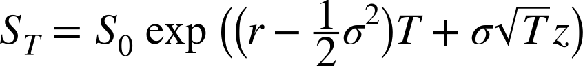
In the BSM model, the index level at maturity is a random variable, given by Equation 1-1 with z being a standard normally distributed random variable.
The following is an algorithmic description of the Monte Carlo valuation procedure:
- Draw I (pseudo)random numbers z(i), i ∈ {1, 2, …, I}, from the standard normal distribution.
- Calculate all resulting index levels at maturity ST(i) for given z(i) and Equation 1-1.
- Calculate all inner values of the option at maturity as hT(i) = max(ST(i) – K,0).
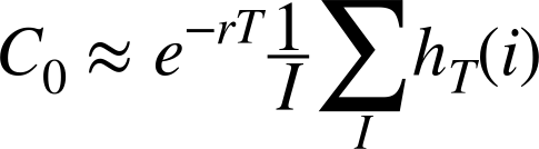
- Estimate the option present value via the Monte Carlo estimator given in Equation 1-2.
We are now going to translate this problem and algorithm into Python code. The reader might follow the single steps by using, for example, IPython—this is, however, not really necessary at this stage.
First, let us start with the parameter values. This is really easy:
S0=100.K=105.T=1.0r=0.05sigma=0.2
Next, the valuation algorithm. Here, we will for the first time use NumPy, which makes life quite easy for our second task:
fromnumpyimport*I=100000z=random.standard_normal(I)ST=S0*exp((r-0.5*sigma**2)*T+sigma*sqrt(T)*z)hT=maximum(ST-K,0)C0=exp(-r*T)*sum(hT)/I
Third, we print the result:
"Value of the European Call Option%5.3f"%C0
The output might be:[4]
Value of the European Call Option 8.019
Three aspects are worth highlighting:
- Syntax
-
The
Pythonsyntax is indeed quite close to the mathematical syntax, e.g., when it comes to the parameter value assignments. - Translation
-
Every mathematical and/or algorithmic statement can generally be translated into a single line of
Pythoncode. - Vectorization
-
One of the strengths of
NumPyis the compact, vectorized syntax, e.g., allowing for 100,000 calculations within a single line of code.
This code can be used in an interactive environment like IPython. However, code that is meant to be reused regularly typically gets organized in so-called modules (or scripts), which are single Python (i.e., text) files with the suffix .py. Such a module could in this case look like Example 1-1 and could be saved as a file named bsm_mcs_euro.py.
## Monte Carlo valuation of European call option# in Black-Scholes-Merton model# bsm_mcs_euro.py#importnumpyasnp# Parameter ValuesS0=100.# initial index levelK=105.# strike priceT=1.0# time-to-maturityr=0.05# riskless short ratesigma=0.2# volatilityI=100000# number of simulations# Valuation Algorithmz=np.random.standard_normal(I)# pseudorandom numbersST=S0*np.exp((r-0.5*sigma**2)*T+sigma*np.sqrt(T)*z)# index values at maturityhT=np.maximum(ST-K,0)# inner values at maturityC0=np.exp(-r*T)*np.sum(hT)/I# Monte Carlo estimator# Result Output"Value of the European Call Option%5.3f"%C0
The rather simple algorithmic example in this subsection illustrates that Python, with its very syntax, is well suited to complement the classic duo of scientific languages, English and Mathematics. It seems that adding Python to the set of scientific languages makes it more well rounded. We have
- English for writing, talking about scientific and financial problems, etc.
- Mathematics for concisely and exactly describing and modeling abstract aspects, algorithms, complex quantities, etc.
- Python for technically modeling and implementing abstract aspects, algorithms, complex quantities, etc.
Mathematics and Python Syntax
There is hardly any programming language that comes as close to mathematical syntax as Python. Numerical algorithms are therefore simple to translate from the mathematical representation into the Pythonic implementation. This makes prototyping, development, and code maintenance in such areas quite efficient with Python.
In some areas, it is common practice to use pseudocode and therewith to introduce a fourth language family member. The role of pseudocode is to represent, for example, financial algorithms in a more technical fashion that is both still close to the mathematical representation and already quite close to the technical implementation. In addition to the algorithm itself, pseudocode takes into account how computers work in principle.
This practice generally has its cause in the fact that with most programming languages the technical implementation is quite “far away” from its formal, mathematical representation. The majority of programming languages make it necessary to include so many elements that are only technically required that it is hard to see the equivalence between the mathematics and the code.
Nowadays, Python is often used in a pseudocode way since its syntax is almost analogous to the mathematics and since the technical “overhead” is kept to a minimum. This is accomplished by a number of high-level concepts embodied in the language that not only have their advantages but also come in general with risks and/or other costs. However, it is safe to say that with Python you can, whenever the need arises, follow the same strict implementation and coding practices that other languages might require from the outset. In that sense, Python can provide the best of both worlds: high-level abstraction and rigorous implementation.
Efficiency and Productivity Through Python
At a high level, benefits from using Python can be measured in three dimensions:
- Efficiency
-
How can
Pythonhelp in getting results faster, in saving costs, and in saving time? - Productivity
-
How can
Pythonhelp in getting more done with the same resources (people, assets, etc.)? - Quality
-
What does
Pythonallow us to do that we could not do with alternative technologies?
A discussion of these aspects can by nature not be exhaustive. However, it can highlight some arguments as a starting point.
Shorter time-to-results
A field where the efficiency of Python becomes quite obvious is interactive data analytics. This is a field that benefits strongly from such powerful tools as IPython and libraries like pandas.
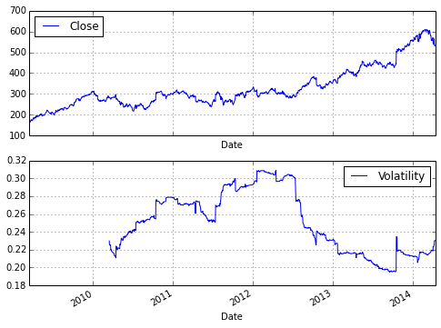
Consider a finance student, writing her master’s thesis and interested in Google stock prices. She wants to analyze historical stock price information for, say, five years to see how the volatility of the stock price has fluctuated over time. She wants to find evidence that volatility, in contrast to some typical model assumptions, fluctuates over time and is far from being constant. The results should also be visualized. She mainly has to do the following:
- Download Google stock price data from the Web.
- Calculate the rolling standard deviation of the log returns (volatility).
- Plot the stock price data and the results.
These tasks are complex enough that not too long ago one would have considered them to be something for professional financial analysts. Today, even the finance student can easily cope with such problems. Let us see how exactly this works—without worrying about syntax details at this stage (everything is explained in detail in subsequent chapters).
First, make sure to have available all necessary libraries:
In[1]:importnumpyasnpimportpandasaspdimportpandas.io.dataasweb
Second, retrieve the data from, say, Google itself:
In[2]:goog=web.DataReader('GOOG',data_source='google',start='3/14/2009',end='4/14/2014')goog.tail()
Out[2]:             Open    High    Low     Close   Volume
        Date
        2014-04-08  542.60  555.00  541.61  554.90  3152406
        2014-04-09  559.62  565.37  552.95  564.14  3324742
        2014-04-10  565.00  565.00  539.90  540.95  4027743
        2014-04-11  532.55  540.00  526.53  530.60  3916171
        2014-04-14  538.25  544.10  529.56  532.52  2568020

        5 rows × 5 columns
Third, implement the necessary analytics for the volatilities:
In[3]:goog['Log_Ret']=np.log(goog['Close']/goog['Close'].shift(1))goog['Volatility']=pd.rolling_std(goog['Log_Ret'],window=252)*np.sqrt(252)
Fourth, plot the results. To generate an inline plot, we use the IPython magic command %matplotlib with the option inline:
In[4]:%matplotlibinlinegoog[['Close','Volatility']].plot(subplots=True,color='blue',figsize=(8,6))
Figure 1-1 shows the graphical result of this brief interactive session with IPython. It can be considered almost amazing that four lines of code suffice to implement three rather complex tasks typically encountered in financial analytics: data gathering, complex and repeated mathematical calculations, and visualization of results. This example illustrates that pandas makes working with whole time series almost as simple as doing mathematical operations on floating-point numbers.
Translated to a professional finance context, the example implies that financial analysts can—when applying the right Python tools and libraries, providing high-level abstraction—focus on their very domain and not on the technical intrinsicalities. Analysts can react faster, providing valuable insights almost in real time and making sure they are one step ahead of the competition. This example of increased efficiency can easily translate into measurable bottom-line effects.
Ensuring high performance
In general, it is accepted that Python has a rather concise syntax and that it is relatively efficient to code with. However, due to the very nature of Python being an interpreted language, the prejudice persists that Python generally is too slow for compute-intensive tasks in finance. Indeed, depending on the specific implementation approach, Python can be really slow. But it does not have to be slow—it can be highly performing in almost any application area. In principle, one can distinguish at least three different strategies for better performance:
- Paradigm
-
In general, many different ways can lead to the same result in
Python, but with rather different performance characteristics; “simply” choosing the right way (e.g., a specific library) can improve results significantly. - Compiling
-
Nowadays, there are several performance libraries available that provide compiled versions of important functions or that compile
Pythoncode statically or dynamically (at runtime or call time) to machine code, which can be orders of magnitude faster; popular ones areCythonandNumba. - Parallelization
-
Many computational tasks, in particular in finance, can strongly benefit from parallel execution; this is nothing special to
Pythonbut something that can easily be accomplished with it.
Performance Computing with Python
Python per se is not a high-performance computing technology. However, Python has developed into an ideal platform to access current performance technologies. In that sense, Python has become something like a glue language for performance computing.
Later chapters illustrate all three techniques in detail. For the moment, we want to stick to a simple, but still realistic, example that touches upon all three techniques.
A quite common task in financial analytics is to evaluate complex mathematical expressions on large arrays of numbers. To this end, Python itself provides everything needed:
In[1]:loops=25000000frommathimport*a=range(1,loops)deff(x):return3*log(x)+cos(x)**2%timeitr=[f(x)forxina]
Out[1]: 1 loops, best of 3: 15 s per loop
The Python interpreter needs 15 seconds in this case to evaluate the function f 25,000,000 times.
The same task can be implemented using NumPy, which provides optimized (i.e., pre-compiled), functions to handle such array-based operations:
In[2]:importnumpyasnpa=np.arange(1,loops)%timeitr=3*np.log(a)+np.cos(a)**2
Out[2]: 1 loops, best of 3: 1.69 s per loop
Using NumPy considerably reduces the execution time to 1.7 seconds.
However, there is even a library specifically dedicated to this kind of task. It is called numexpr, for “numerical expressions.” It compiles the expression to improve upon the performance of NumPy’s general functionality by, for example, avoiding in-memory copies of arrays along the way:
In[3]:importnumexprasnene.set_num_threads(1)f='3 * log(a) + cos(a) ** 2'%timeitr=ne.evaluate(f)
Out[3]: 1 loops, best of 3: 1.18 s per loop
Using this more specialized approach further reduces execution time to 1.2 seconds. However, numexpr also has built-in capabilities to parallelize the execution of the respective operation. This allows us to use all available threads of a CPU:
In[4]:ne.set_num_threads(4)%timeitr=ne.evaluate(f)
Out[4]: 1 loops, best of 3: 523 ms per loop
This brings execution time further down to 0.5 seconds in this case, with two cores and four threads utilized. Overall, this is a performance improvement of 30 times. Note, in particular, that this kind of improvement is possible without altering the basic problem/algorithm and without knowing anything about compiling and parallelization issues. The capabilities are accessible from a high level even by nonexperts. However, one has to be aware, of course, of which capabilities exist.
The example shows that Python provides a number of options to make more out of existing resources—i.e., to increase productivity. With the sequential approach, about 21 mn evaluations per second are accomplished, while the parallel approach allows for almost 48 mn evaluations per second—in this case simply by telling Python to use all available CPU threads instead of just one.
From Prototyping to Production
Efficiency in interactive analytics and performance when it comes to execution speed are certainly two benefits of Python to consider. Yet another major benefit of using Python for finance might at first sight seem a bit subtler; at second sight it might present itself as an important strategic factor. It is the possibility to use Python end to end, from prototyping to production.
Today’s practice in financial institutions around the globe, when it comes to financial development processes, is often characterized by a separated, two-step process. On the one hand, there are the quantitative analysts (“quants”) responsible for model development and technical prototyping. They like to use tools and environments like Matlab and R that allow for rapid, interactive application development. At this stage of the development efforts, issues like performance, stability, exception management, separation of data access, and analytics, among others, are not that important. One is mainly looking for a proof of concept and/or a prototype that exhibits the main desired features of an algorithm or a whole application.
Once the prototype is finished, IT departments with their developers take over and are responsible for translating the existing prototype code into reliable, maintainable, and performant production code. Typically, at this stage there is a paradigm shift in that languages like C++ or Java are now used to fulfill the requirements for production. Also, a formal development process with professional tools, version control, etc. is applied.
This two-step approach has a number of generally unintended consequences:
- Inefficiencies
- Prototype code is not reusable; algorithms have to be implemented twice; redundant efforts take time and resources.
- Diverse skill sets
- Different departments show different skill sets and use different languages to implement “the same things.”
- Legacy code
- Code is available and has to be maintained in different languages, often using different styles of implementation (e.g., from an architectural point of view).
Using Python, on the other hand, enables a streamlined end-to-end process from the first interactive prototyping steps to highly reliable and efficiently maintainable production code. The communication between different departments becomes easier. The training of the workforce is also more streamlined in that there is only one major language covering all areas of financial application building. It also avoids the inherent inefficiencies and redundancies when using different technologies in different steps of the development process. All in all, Python can provide a consistent technological framework for almost all tasks in financial application development and algorithm implementation.
Conclusions
Python as a language—but much more so as an ecosystem—is an ideal technological framework for the financial industry. It is characterized by a number of benefits, like an elegant syntax, efficient development approaches, and usability for prototyping and production, among others. With its huge amount of available libraries and tools, Python seems to have answers to most questions raised by recent developments in the financial industry in terms of analytics, data volumes and frequency, compliance, and regulation, as well as technology itself. It has the potential to provide a single, powerful, consistent framework with which to streamline end-to-end development and production efforts even across larger financial institutions.
Further Reading
There are two books available that cover the use of Python in finance:
- Fletcher, Shayne and Christopher Gardner (2009): Financial Modelling in Python. John Wiley & Sons, Chichester, England.
- Hilpisch, Yves (2015): Derivatives Analytics with Python. Wiley Finance, Chichester, England. http://derivatives-analytics-with-python.com.
The quotes in this chapter are taken from the following resources:
- Crosman, Penny (2013): “Top 8 Ways Banks Will Spend Their 2014 IT Budgets.” Bank Technology News.
- Deutsche Börse Group (2008): “The Global Derivatives Market—An Introduction.” White paper.
- Ding, Cubillas (2010): “Optimizing the OTC Pricing and Valuation Infrastructure.” Celent study.
- Lewis, Michael (2014): Flash Boys. W. W. Norton & Company, New York.
- Patterson, Scott (2010): The Quants. Crown Business, New York.
[1] Python, for example, is a major language used in the Master of Financial Engineering program at Baruch College of the City University of New York (cf. http://mfe.baruch.cuny.edu).
[2] Cf. http://wiki.python.org/moin/BeginnersGuide, where you will find links to many valuable resources for both developers and nondevelopers getting started with Python.
[3] Chapter 8 provides an example for the benefits of using modern GPGPUs in the context of the generation of random numbers.
[4] The output of such a numerical simulation depends on the pseudorandom numbers used. Therefore, results might vary.
Get Python for Finance now with the O’Reilly learning platform.
O’Reilly members experience books, live events, courses curated by job role, and more from O’Reilly and nearly 200 top publishers.

