Apply Formatting
Pivot tables usually look pretty awful when you first create them. In the preceding example, the ProductName columns are very wide at first (see Figure 13-3). I adjusted them manually to get a nice screenshot for Figure 13-5, but if you click Refresh Data the columns revert to wide.
There are two ways to change pivot table formatting :
Set table formatting manually.
Apply an autoformat to the table.
To set the formatting manually:
Select the pivot table and choose Pivot Table → Table Options from the pivot table toolbar. Excel displays Figure 13-6.
Clear the AutoFormat Table option and click OK to close the dialog.
Set column widths and cell formatting in the usual way. Those changes are now preserved when you refresh the table.
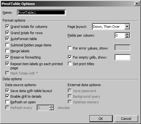
Figure 13-6. Deselect AutoFormat Table to preserve manual formatting
Tip
The Preserve Formatting option in Figure 13-6 preserves cell formatting, such as fonts and colors. That option is on by default, so you don’t have to change it.
Even with reasonable column widths, the pivot table in Figure 13-5 isn’t as readable as it could be. To autoformat the table:
Select the pivot table and click the Format Report button on the PivotTable toolbar. Excel displays the AutoFormat dialog box.
Choose a format and click OK to apply it to the table. Figure 13-7 shows the result.
Figure 13-7. Apply an autoformat to create a nice-looking report
Get Programming Excel with VBA and .NET now with the O’Reilly learning platform.
O’Reilly members experience books, live events, courses curated by job role, and more from O’Reilly and nearly 200 top publishers.

