Let’s Make Some Graphs!
The GD::Graph package was written by Martien Verbruggen. It should run on any operating system on which the GD module is available. GD::Graph uses the GD module for all of its drawing and file primitives, and also relies on the GD::TextUtil package. Both packages are available from CPAN at http://www.cpan.org/authors/id/MVERB/.
Graph construction with GD::Graph can be broken into three
phases. First you need to gather the data, parse it, and organize it
in a form that you can pass to the graph drawing routines. Then you
set the attributes of the graph such that it will come out the way you
want it. Finally, you draw the graph with the plot( ) method.
The data for the graph must be in a very particular form before you plot the graph. The plotting methods expect a reference to an array, where the first element is a reference to an anonymous array of the x-axis values, and any subsequent elements are data sets to be plotted against the y axis. A sample data collection looks like this:
#!/usr/bin/perl -w

use GD;      # for font names
use GD::Graph::lines;
my @data = ( [ qw(1955 1956 1957 1958
                  1959 1960 1961 1962
                  1963 1964 1965 1966
                  1967 1968 1969 1970
                  1971 1972 1973 ) ],   # timespan of data

             # thousands of people in New York
             [ 2,  5,  16.8,  18, 19, 22.6, 26, 32, 34, 39,
               43, 48, 49, 49, 54.2, 58, 68, 72, 79 ],

             # thousands of people in SF
             [ 11,  18,  29.4,  35.7, 36, 38.2, 36, 41, 45, 49,
               50, 51, 51.4, 52.6, 53.2, 54, 67, 73, 78 ],

             # thousands of people in Peoria
             [ 5,  8,  24,  32, 37, 40, 50, 55, 61, 63,
               61, 60, 65.5, 68, 71, 69, 73, 73.5, 78, 78.5],

             # thousands of people in Seattle
             [ 4.25,  8.9, 19, 21, 25, 24, 27, 29, 33, 35,
               41, 40, 45, 42, 44, 49, 51, 58, 61, 66],

             # thousands of people in Tangiers
             [ 2,  11,  9,  9.2, 9.8, 10.1, 8.2, 8.5, 9, 7,
               6, 5.5, 6.5, 5.2, 4.5, 4.2, 4, 3, 2, 1 ],

             # thousands of people in Moscow
             [ 3.5,  8,  22,  22.5, 23, 25, 25, 25, 26, 21,
               20, 19.2, 19.7, 21, 18, 23, 17, 12, 10, 5],

             # thousands of people in Istanbul
             [ 6.5,  12.8,  31.7,  34, 32, 29, 19, 20.5, 28, 35,
              34, 33, 30, 28, 25, 21, 20, 16, 11, 9]
     );
You can use the GD::Graph::Data module to help reorganize your
data if it’s in a different format (an example is shown later in this
section). If your data set doesn’t have data for each point, use
undef for those points without
data.
GD::Graph implements eight different types of graphs: area, bars, hbars, lines, lines and points, points, mixed, and pie graphs (see Figure 4-1 for samples of each of these graph types). To create a new graph that connects all the data points with different colored lines, start with:
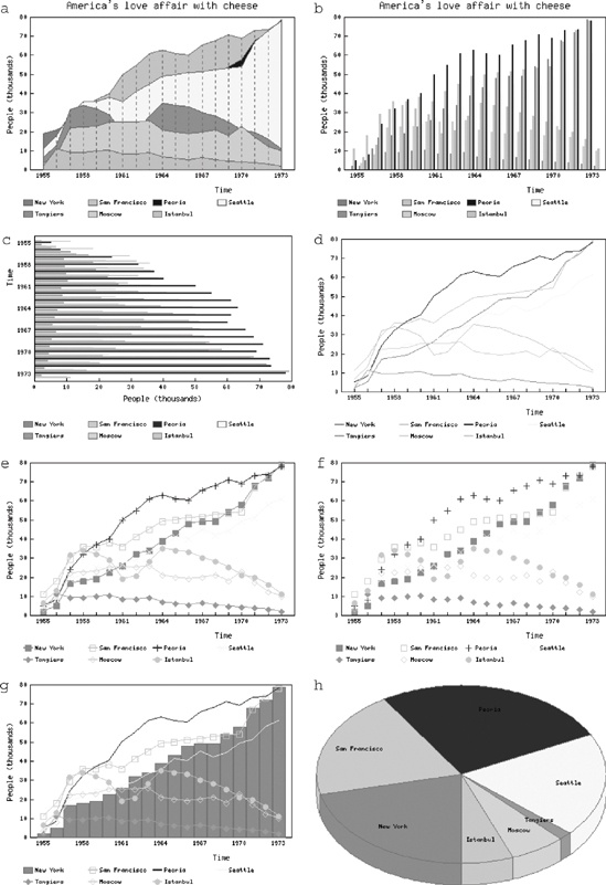
my $graph = new GD::Graph::lines( );
Each graph type has many attributes that may be used to control
the format, color, and content of the graph. Use the set( ) method to configure your
graph:
$graph->set(
        title             => "America's love affair with cheese",
        x_label           => 'Time',
        y_label           => 'People (thousands)',
        y_max_value       => 80,
        y_tick_number     => 8,
        x_all_ticks       => 1,
        y_all_ticks       => 1,
        x_label_skip      => 3,
    );

$graph->set_legend_font(GD::gdFontTiny);
$graph->set_legend('New York', 'San Francisco', 'Peoria',
                    'Seattle', 'Tangiers', 'Moscow', 'Istanbul');
Finally, draw the graph with the plot(
) method, which creates a graph and returns a GD object. Use
the GD object to create a PNG image:
my $gd = $graph->plot( \@data );

open OUT, ">cheese.png" or die "Couldn't open for output: $!";
binmode(OUT);
print OUT $gd->png( );
close OUT;
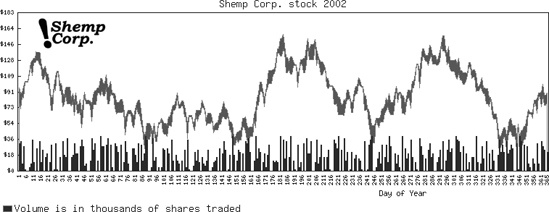
The mixed chart is a special type that combines different charting methods within the same frame. In the next example, we’ll use a mixed area-and-bars chart to communicate a year’s worth of stock activity for the fictional Shemp company. It graphs three values for each day in the year: the stock’s high value, low value, and volume. Then we’ll do a little graphical sleight-of-hand to make the high and low values look like one jagged line that varies in thickness to demonstrate the volatility of the price—the thicker the line, the greater the difference between the high and low. The output is shown in Figure 4-2.
This example also shows the use of the GD::Graph::Data module as a cleaner alternative for specifying chart data. First we create a new GD::Graph::Data object, which can read in data from a previously created file:
#!/usr/bin/perl -w
#
# A mixed stock graph

use strict;
use GD;
use GD::Graph::Data;
use GD::Graph::mixed;

# Read in the data from a file

my $data = GD::Graph::Data->new( );
$data->read(file => 'stock_data.dat');
where the stock_data.dat file is in the format:
1       96      80      32
2       89      72      34
3       90      86      8
4       98      84      28
5       104     103     2
...etc...
The default delimiter between each field of this file is a tab;
you can set the delimiter parameter
to use a different delimiter string. The first field on each line is
the x value, followed by the y values for high, low, and volume. Look
at the documentation for the GD::Graph::Data module for more methods
to help you manage data.
The next step is to create the graph and set the various
attributes. The types attribute
assigns a different chart type to each of the data sets. The dclrs attribute assigns a color to each data
set. For an area graph, the space underneath the curve of the graph is
shaded with the specified color. The daily high value is drawn first
in solid red, followed by the daily low in white. The low value acts
as a mask, so that only the y values between the low and the high are
drawn in red. The daily volume is charted along the bottom as a blue
bar graph.
my $graph = new GD::Graph::mixed(900, 300) or die "Can't create graph!";

# Set the general attributes

$graph->set(
        title             => "Shemp Corp. stock 2002",
        types             => [qw(area area bars)],
        dclrs             => [qw(red white blue)],
        transparent       => 0,
);

# Set the attributes for the x-axis

$graph->set(
        x_label           => 'Day of Year',
        x_label_skip      => 5,
        x_labels_vertical => 1,
);
The range of y-axis values is determined by a function of the
GD::Graph::Data module that returns the minimum and maximum values of
each data set. When plotting each y-axis label, use a special feature
of the y_number_format attribute.
If this attribute is set to a reference to a subroutine, each y-axis
label is passed to the routine, and the returned value is used as the
label. In this case, we add a dollar sign to each label and round off
fractional values:
$graph->set(
        y_max_value       => ($data->get_min_max_y_all( ))[1]+25,
        y_tick_number     => 10,
        y_all_ticks       => 1,
        y_number_format   => sub { '$'.int(shift); },
);
The legend is a string that describes each
of the various data sets. Here we only need to make a note about the
scale used for the volume graph, so the legends for the first two data
sets are assigned undef.
# Set the legend

$graph->set_legend(undef, undef, 'Volume is in thousands of shares traded');
$graph->set_legend_font(gdLargeFont);
$graph->set(legend_placement => 'BL');

# Plot the data

my $gd = $graph->plot( $data ) or die "Can't plot graph";
If you wanted to add a little graphical logo to a corner of the
graph, you would typically use the logo attribute to assign a PNG file for the
logo. However, the copyResized( )
method (used by GD::Graph to apply logos) was broken in the beta
version of the GD module I was using when I wrote this book. It’s easy
enough to reimplement logo insertion with GD, though. Since we’ve
already plotted the graph, we have a GD object ready for use:
my $logo = GD::Image->newFromPng('shempcorp.png');
my ($w, $h) = $logo->getBounds( );
$gd->copy($logo, 50, 25, 0, 0, $w, $h);

# Write the PNG

print $gd->png( );
The pie chart is a bit different from the other graph types. The next example uses pie charts as elements that are pieced together into a larger information graphic using GD. The five pie charts are drawn with GD::Chart.
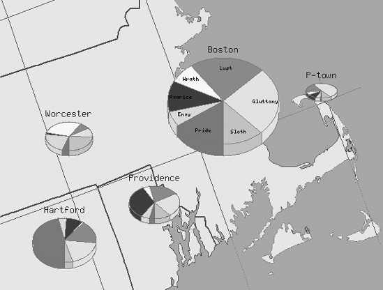
We’ve collected data on the seven deadly sins in five New England cities, each of which will have its own pie chart showing the particular weaknesses of that community. Each pie chart will be placed near the city on the map and is sized proportionately according to the population of the city (see Figure 4-3).
To do this, we first set up a data structure that encapsulates the data for each city. A big hash works fine for this:
#!/usr/bin/perl -w
#
# Pie charts on a map

use GD;
use GD::Graph::pie;

# The sins

my $pie_labels = [ qw(Pride Envy Avarice
                      Wrath Lust Gluttony Sloth)];
my %cities = (
    'Boston' => { size => 175,
                  x => 260,
                  y => 100,
                 data => [24, 9, 18, 12, 35, 40, 19] },
    'Providence' => {
                  size => 80,
                  x => 200,
                  y => 300,
                  data => [5, 10, 60, 8, 35, 40, 19] },
    'Hartford' => {
                  size => 100,
                  x => 50,
                  y => 350,
                  data => [100, 9, 18, 2, 35, 40, 9] },
    'Worcester' => {
                  size => 75,
                  x => 70,
                  y => 200,
                  data => [2, 9, 1, 12, 3, 4, 10] },
    'P-town' => {
                  size => 50,
                  x => 475,
                  y => 140,
                  data => [2, 9, 18, 12, 35, 90, 19] },
);
Next we read the previously created image of the map into a new GD image. Then, we loop through the keys of the city hash and create a new pie graph for each data set.
my $map = GD::Image->newFromPng('map.png');

# Loop through the cities, creating a graph for each

foreach my $city (keys(%cities)) {
    my $size = $cities{$city}->{'size'};

    my $graph = new GD::Graph::pie($size,$size)
        or die "Can't create graph!";
    $graph->set( transparent    => 1,
                 suppress_angle => 360*($size<150),
                '3d'           => 1,
                 title          => $city,
    );
The suppress_angle attribute
is unique to the pie chart type. If this attribute is non-zero, the
label for a particular piece of pie is not drawn if the angle is less
than this value. If the angle is 360, no pie labels are produced. This
code suppresses labels for pie charts that are smaller than 150 pixels
in diameter.
Next, we plot the pie chart, then place it on the map with GD’s
copy( ) method.
# Plot the graph

    my $gd = $graph->plot([ $pie_labels,
                            $cities{$city}->{'data'} ])
        or die "Can't plot graph";

    # Copy the graph onto the map at the specified coordinate

    my ($w, $h) = $graph->gd( )->getBounds( );
    $map->copy($graph->gd( ),
               $cities{$city}->{'x'},
               $cities{$city}->{'y'},
               0, 0, $w, $h);
}
When all five pies have been added, we print out the composite map as a PNG to STDOUT.
# Print the map to STDOUT

print $map->png( );
The following section collects the concepts developed here into a complete working application.
Get Perl Graphics Programming now with the O’Reilly learning platform.
O’Reilly members experience books, live events, courses curated by job role, and more from O’Reilly and nearly 200 top publishers.

