APPENDIX A
Distributions
The distribution of a variable gives the relative number of times each outcome occurs in a given number of trials. The function that describes the probability that a given value will occur is the probability density function. A completely equivalent characterization is the cumulative probability that a given value or any smaller value will occur. This is called the cumulative distribution function (sometimes just referred to as the distribution function).
EXAMPLE
One of the most useful distributions is the normal distribution (also known as the Gaussian distribution or the bell curve). This is a continuous distribution that describes many situations. It is also mathematically tractable. Its probability density is given by
(A.1)
This has two parameters: a location parameter, µ and a scale parameter, σ.
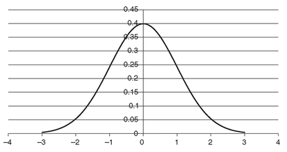
An example of this distribution is shown in
Figure A.1.
FIGURE A.1 A Normal Distribution with
µ = 0,
σ = 1
For a normal distribution, approximately 68 percent of outcomes are within one standard deviation of the mean, 95 percent are within two standard deviations, and 99 percent are within three standard deviations.
Most other distributions need more parameters to fully describe them.
MOMENTS AND THE “SHAPE” OF DISTRIBUTIONS
The mean and the variance provide ...


