MongoDB Applied Design Patterns

Chapter 4. Operational Intelligence

The first use cases we’ll explore lie in the realm of operational intelligence, the techniques of converting transactional data to actionable information in a business setting. Of course, the starting point for any of these techniques is getting the raw transactional data into your data store. Our first use case, Storing Log Data, deals with this part of the puzzle.

Once you have the data, of course, the first priority is to generate actionable reports on that data, ideally in real time with the data import itself. We address the generation of these reports in real time in Pre-Aggregated Reports.

Finally, we’ll explore the use of more traditional batch aggregation in Hierarchical Aggregation to see how MongoDB can be used to generate reports at multiple layers of your analytics hierarchy.

Storing Log Data

The starting point for any analytics system is the raw “transactional” data. To give a feel for this type of problem, we’ll examine the particular use case of storing event data in MongoDB that would traditionally be stored in plain-text logfiles. Although plain-text logs are accessible and human-readable, they are difficult to use, reference, and analyze, frequently being stored on a server’s local filesystem in an area that is generally inaccessible to the business analysts who need these data.

Solution Overview

The solution described here assumes that each server generating events can access the MongoDB instance and has read/write access to some database on that instance. Furthermore, we assume that the query rate for logging data is significantly lower than the insert rate for log data.

Note

This case assumes that you’re using a standard uncapped collection for this event data, unless otherwise noted. See Capped collections for another approach to aging out old data.

Schema Design

The schema for storing log data in MongoDB depends on the format of the event data that you’re storing. For a simple example, you might consider standard request logs in the combined format from the Apache HTTP Server. A line from these logs may resemble the following:

127.0.0.1 - frank [10/Oct/2000:13:55:36 -0700] "GET /apache_pb.gif HTTP/1.0" ...

The simplest approach to storing the log data would be putting the exact text of the log record into a document:

{
  _id: ObjectId(...),
 line: '127.0.0.1 - frank [10/Oct/2000:13:55:36 -0700] "GET /apache_pb.gif ...
}

Although this solution does capture all data in a format that MongoDB can use, the data is neither particularly useful nor efficient. For example, if you need to find events on the same page, you would need to use a regular expression query, which would require a full scan of the collection. A better approach is to extract the relevant information from the log data into individual fields in a MongoDB document.

When designing the structure of that document, it’s important to pay attention to the data types available for use in BSON, the MongoDB document format. Choosing your data types wisely can have a significant impact on the performance and capability of the logging system. For instance, consider the date field. In the previous example, [10/Oct/2000:13:55:36 -0700] is 28 bytes long. If you store this with the UTC timestamp BSON type, you can convey the same information in only 8 bytes.

Additionally, using proper types for your data also increases query flexibility. If you store date as a timestamp, you can make date range queries, whereas it’s very difficult to compare two strings that represent dates. The same issue holds for numeric fields; storing numbers as strings requires more space and is more difficult to query.

Consider the following document that captures all data from the log entry:

{
     _id: ObjectId(...),
     host: "127.0.0.1",
     logname: null,
     user: 'frank',
     time:  ISODate("2000-10-10T20:55:36Z"),
     request: "GET /apache_pb.gif HTTP/1.0",
     status: 200,
     response_size: 2326,
     referrer: "[http://www.example.com/start.html](http://www.example.com/...",
     user_agent: "Mozilla/4.08 [en] (Win98; I ;Nav)"
}

The is better, but it’s quite a large document. When extracting data from logs and designing a schema, you should also consider what information you can omit from your log tracking system. In most cases, there’s no need to track all data from an event log. To continue this example, here the most crucial information may be the host, time, path, user agent, and referrer, as in the following example document:

{
     _id: ObjectId(...),
     host: "127.0.0.1",
     time:  ISODate("2000-10-10T20:55:36Z"),
     path: "/apache_pb.gif",
     referer: "[http://www.example.com/start.html](http://www.example.com/...",
     user_agent: "Mozilla/4.08 [en] (Win98; I ;Nav)"
}

Depending on your storage and memory requirements, you might even consider omitting explicit time fields, since the BSON ObjectId implicitly embeds its own creation time:

 {
      _id: ObjectId('...'),
      host: "127.0.0.1",
      path: "/apache_pb.gif",
      referer: "[http://www.example.com/start.html](http://www.example.com/...",
      user_agent: "Mozilla/4.08 [en] (Win98; I ;Nav)"
 }

Operations

In this section, we’ll describe the various operations you’ll need to perform on the logging system, paying particular attention to the appropriate use of indexes and MongoDB-specific features.

Inserting a log record

The primary performance concerns for event-logging systems are:

• How many inserts per second it can support, which limits the event throughput
• How the system will manage the growth of event data, particularly in the case of a growth in insert activity

In designing our system, we’ll primarily focus on optimizing insertion speed, while still addressing how we manage event data growth. One decision that MongoDB allows you to make when performing updates (such as event data insertion) is whether you want to trade off data safety guarantees for increased insertion speed. This section will explore the various options we can tweak depending on our tolerance for event data loss.

Write concern

MongoDB has a configurable write concern. This capability allows you to balance the importance of guaranteeing that all writes are fully recorded in the database with the speed of the insert.

For example, if you issue writes to MongoDB and do not require that the database issue any response, the write operations will return very fast (since the application needs to wait for a response from the database) but you cannot be certain that all writes succeeded. Conversely, if you require that MongoDB acknowledge every write operation, the database will not return as quickly but you can be certain that every item will be present in the database.

The proper write concern is often an application-specific decision, and depends on the reporting requirements and uses of your analytics application.

In the examples in this section, we will assume that the following code (or something similar) has set up an event from the Apache Log. In a real system, of course, we would need code to actually parse the log and create the Python dict shown here:

>>> import bson
>>> import pymongo
>>> from datetime import datetime
>>> conn = pymongo.Connection()
>>> db = conn.event_db
>>> event = {
...    _id: bson.ObjectId(),
...    host: "127.0.0.1",
...    time:  datetime(2000,10,10,20,55,36),
...    path: "/apache_pb.gif",
...    referer: "[http://www.example.com/start.html](http://www.example.com/...",
...    user_agent: "Mozilla/4.08 [en] (Win98; I ;Nav)"
...}

The following command will insert the event object into the events collection:

>>> db.events.insert(event, w=0)

By setting w=0, you do not require that MongoDB acknowledge receipt of the insert. Although this is the fastest option available to us, it also carries with it the risk that you might lose a large number of events before you notice.

If you want to ensure that MongoDB acknowledges inserts, you can omit the w=0 argument, or pass w=1 (the default) as follows:

>>> db.events.insert(event)
>>> # Alternatively, you can do this
>>> db.events.insert(event, w=1)

MongoDB also supports a more stringent level of write concern, if you have a lower tolerance for data loss. MongoDB uses an on-disk journal file to persist data before writing the updates back to the “regular” data files.

Since journal writes are significantly slower than in-memory updates (which are, in turn, much slower than “regular” data file updates), MongoDB batches up journal writes into “group commits” that occur every 100 ms unless overridden in your server settings. What this means for the application developer is that, on average, any individual writes with j=True will take around 50 ms to complete, which is generally even more time than it would take to replicate the data to another server. If you want to ensure that MongoDB not only acknowledges receipt of a write operation but also commits the write operation to the on-disk journal before returning successfully to the application, you can use the j=True option:

>>> db.events.insert(event, j=True)

It’s important to note that the journal does not protect against any failure in which the disk itself might fail, since in that case the journal file itself can be corrupted. Replication, however, does protect against single-server failures, and is the recommended way to achieve real durability.

Note

j=True requires acknowledgment from the server, so w=1 is implied unless you explicitly set w=N with N greater than 1.

You can require that MongoDB replicate the data to multiple secondary replica set members before returning:

>>> db.events.insert(event, w=2)

This will force your application to acknowledge that the data has replicated to two members of the replica set. You can combine options as well:

>>> db.events.insert(event, j=True, w=2)

In this case, your application will wait for a successful journal commit and a replication acknowledgment. This is the safest option presented in this section, but it is the slowest. There is always a trade-off between safety and speed.

Bulk inserts

If possible, you should use bulk inserts to insert event data. All write concern options apply to bulk inserts, but you can pass multiple events to the insert() method at once. Batch inserts allow MongoDB to distribute the performance penalty incurred by more stringent write concern across a group of inserts.

If you’re doing a bulk insert and do get an error (either a network interruption or a unique key violation), your application will need to handle the possibility of a partial bulk insert. If your particular use case doesn’t care about missing a few inserts, you can add the continue_on_error=True argument to insert, in which case the insert will insert as many documents as possible, and report an error on the last insert that failed.

If you use continue_on_error=True and multiple inserts in your batch fail, your application will only receive information on the last insert to fail. The take-away? You can sometimes amortize the overhead of safer writes by using bulk inserts, but this technique brings with it another set of concerns as well.

Finding all events for a particular page

The value in maintaining a collection of event data derives from being able to query that data to answer specific questions. You may have a number of simple queries that you may use to analyze these data.

As an example, you may want to return all of the events associated with a specific value of a field. Extending the Apache access log example, a common case would be to query for all events with a specific value in the path field. This section contains a pattern for returning data and optimizing this operation.

In this case, you’d use a query that resembles the following to return all documents with the /apache_pb.gif value in the path field:

>>> q_events = db.events.find({'path': '/apache_pb.gif'})

Of course, if you want this query to perform well, you’ll need to add an index on the path field:

>>> db.events.ensure_index('path')

Aside: managing index size

One thing you should keep in mind when you’re creating indexes is the size they take up in RAM. When an index is accessed randomly, as in the case here with our index on path, the entire index needs to be resident in RAM. In this particular case, the total number of distinct paths is typically small in relation to the number of documents, which will limit the space that the index requires.

To actually see the size of an index, you can use the collstats database command:

>>> db.command('collstats', 'events')['indexSizes']

There is actually another type of index that doesn’t take up much RAM, and that’s a right-aligned index. Right-aligned refers to the access pattern of a regular index, not a special MongoDB index type: in this case, most of the queries that use the index focus on the largest (or smallest) values in the index, so most of the index is never actually used. This is often the case with time-oriented data, where you tend to query documents from the recent past. In this case, only a very thin “sliver” of the index is ever resident in RAM at a particular time, so index size is of much less concern.

Finding all the events for a particular date

Another operation we might wish to do is to query the event log for all events that happened on a particular date, perhaps as part of a security audit of suspicious activity. In this case, we’ll use a range query:

>>> q_events = db.events.find('time':
...     { '$gte':datetime(2000,10,10),'$lt':datetime(2000,10,11)})

This query selects documents from the events collection where the value of the time field represents a date that is on or after (i.e., $gte) 2000-10-10 but before (i.e., $lt) 2000-10-11. Here, an index on the time field would optimize performance:

>>> db.events.ensure_index('time')

Note that this is a right-aligned index so long as our queries tend to focus on the recent history.

Finding all events for a particular host/date

Expanding on our “security audit” example, suppose we isolated the incident to a particular server and wanted to look at the activity for only a single server on a particular date. In this case, we’d use a query that resembles the following:

>>> q_events = db.events.find({
...     'host': '127.0.0.1',
...     'time': {'$gte':datetime(2000,10,10),'$lt':datetime(2000,10,11)}
... })

The indexes you use may have significant implications for the performance of these kinds of queries. For instance, you can create a compound index on the time-host field pair (noting that order matters), using the following command:

>>> db.events.ensure_index([('time', 1), ('host', 1)])

To analyze the performance for the above query using this index, MongoDB provides the explain() method. In Python for instance, we can execute q_events.explain() in a console. This will return something that resembles:

{ ..
  u'cursor': u'BtreeCursor time_1_host_1',
  u'indexBounds': {u'host': [[u'127.0.0.1', u'127.0.0.1']],
  u'time': [
      [ datetime.datetime(2000, 10, 10, 0, 0),
        datetime.datetime(2000, 10, 11, 0, 0)]]
  },
  ...
  u'millis': 4,
  u'n': 11,
  u'nscanned': 1296,
  u'nscannedObjects': 11,
  ... }

This query had to scan 1,296 items from the index to return 11 objects in 4 milliseconds. Conversely, you can test a different compound index with the host field first, followed by the time field. Create this index using the following operation:

>>> db.events.ensure_index([('host', 1), ('time', 1)])

Now, explain() tells us the following:

{ ...
  u'cursor': u'BtreeCursor host_1_time_1',
  u'indexBounds': {u'host': [[u'127.0.0.1', u'127.0.0.1']],
  u'time': [[datetime.datetime(2000, 10, 10, 0, 0),
      datetime.datetime(2000, 10, 11, 0, 0)]]},
  ...
  u'millis': 0,
  u'n': 11,
  ...
  u'nscanned': 11,
  u'nscannedObjects': 11,
  ...
}

Here, the query had to scan 11 items from the index before returning 11 objects in less than a millisecond. Although the index order has an impact on query performance, remember that index scans are much faster than collection scans, and depending on your other queries, it may make more sense to use the { time: 1, host: 1 } index depending on usage profile.

Rules of index design

MongoDB indexes are stored in a data structure known as a B-tree. The details are beyond our scope here, but what you need to understand as a MongoDB user is that each index is stored in sorted order on all the fields in the index. For an index to be maximally efficient, the key should look just like the queries that use the index. Ideally, MongoDB should be able to traverse the index to the first document that the query returns and sequentially walk the index to find the rest.

Because of this sorted B-tree structure, then, the following rules will lead to efficient indexes:

• Any fields that will be queried by equality should occur first in the index definition.
• Fields used to sort should occur next in the index definition. If multiple fields are being sorted (such as (last_name, first_name), then they should occur in the same order in the index definition.
• Fields that are queried by range should occur last in the index definition.

This leads to some unfortunate circumstances where our index cannot be used optimally:

• Whenever we have a range query on two or more properties, they cannot both be used effectively in the index.
• Whenever we have a range query combined with a sort on a different property, the index is somewhat less efficient than when doing a range and sort on the same property set.

In such cases, the best approach is to test with representative data, making liberal use of explain(). If you discover that the MongoDB query optimizer is making a bad choice of index (perhaps choosing to reduce the number of entries scanned at the expense of doing a large in-memory sort, for instance), you can also use the hint() method to tell it which index to use.

Counting requests by day and page

Finding requests is all well and good, but more frequently we need to count requests, or perform some other aggregate operation on them during analysis. Here, we’ll describe how you can use MongoDB’s aggregation framework, introduced in version 2.1, to select, process, and aggregate results from a large number of documents for powerful ad hoc queries. In this case, we’ll count the number of requests per resource (i.e., page) per day in the last month.

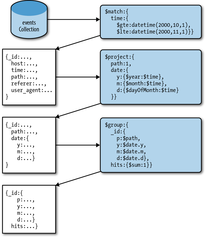
To use the aggregation framework, we need to set up a pipeline of operations. In this case, our pipeline looks like Figure 4-1 and is implemented by the database command shown here:

>>> result = db.command('aggregate', 'events', pipeline=[
...         {  '$match': {   
...               'time': {
...                   '$gte': datetime(2000,10,1),
...                   '$lt':  datetime(2000,11,1) } } },
...         {  '$project': {  
...                 'path': 1,
...                 'date': {
...                     'y': { '$year': '$time' },
...                     'm': { '$month': '$time' },
...                     'd': { '$dayOfMonth': '$time' } } } },
...         { '$group': {  
...                 '_id': {
...                     'p':'$path',
...                     'y': '$date.y',
...                     'm': '$date.m',
...                     'd': '$date.d' },
...                 'hits': { '$sum': 1 } } },
...         ])

This command aggregates documents from the events collection with a pipeline that:

Uses the $match operation to limit the documents that the aggregation framework must process. $match is similar to a find() query. This operation selects all documents where the value of the time field represents a date that is on or after (i.e., $gte) 2000-10-10 but before (i.e., $lt) 2000-10-11.

Uses the $project operator to limit the data that continues through the pipeline. This operator:

• Selects the path field.
• Creates a y field to hold the year, computed from the time field in the original documents.
• Creates an m field to hold the month, computed from the time field in the original documents.
• Creates a d field to hold the day, computed from the time field in the original documents.

Uses the $group operator to create new computed documents. This step will create a single new document for each unique path/date combination. The documents take the following form:

• The _id field holds a subdocument with the content’s path field from the original documents in the p field, with the date fields from the $project as the remaining fields.
• The hits field uses the $sum statement to increment a counter for every document in the group. In the aggregation output, this field holds the total number of documents at the beginning of the aggregation pipeline with this unique date and path.

Figure 4-1. Aggregation pipeline

In sharded environments, the performance of aggregation operations depends on the shard key. Ideally, all the items in a particular $group operation will reside on the same server.

Although this distribution of documents would occur if you chose the time field as the shard key, a field like path also has this property and is a typical choice for sharding. See Sharding Concerns for additional recommendations concerning sharding.

SQL equivalents

To translate statements from the aggregation framework to SQL, you can consider the $match equivalent to WHERE, $project to SELECT, and $group to GROUP BY.

In order to optimize the aggregation operation, you must ensure that the initial $match query has an index. In this case, the command would be simple, and it’s an index we already have:

>>> db.events.ensure_index('time')

If you have already created a compound index on the time and host (i.e., { time: 1, host, 1 },) MongoDB will use this index for range queries on just the time field. In situations like this, there’s no benefit to creating an additional index for just time.

Sharding Concerns

Eventually, your system’s events will exceed the capacity of a single event logging database instance. In these situations you will want to use a shard cluster, which takes advantage of MongoDB’s automatic sharding functionality. In this section, we introduce the unique sharding concerns for the event logging use case.

Limitations

In a sharded environment, the limitations on the maximum insertion rate are:

• The number of shards in the cluster
• The shard key you choose

Because MongoDB distributes data using chunks based on ranges of the shard key, the choice of shard key can control how MongoDB distributes data and the resulting systems’ capacity for writes and queries.

Ideally, your shard key should have two characteristics:

• Insertions are balanced between shards
• Most queries can be routed to a subset of the shards to be satisfied

Here are some initially appealing options for shard keys, which on closer examination, fail to meet at least one of these criteria:

Timestamps

Shard keys based on the timestamp or the insertion time (i.e., the ObjectId) end up all going in the “high” chunk, and therefore to a single shard. The inserts are not balanced.

Hashes

If the shard key is random, as with a hash, then all queries must be broadcast to all shards. The queries are not routeable.

We’ll now examine these options in more detail.

Option 1: Shard by time

Although using the timestamp, or the ObjectId in the _id field, would distribute your data evenly among shards, these keys lead to two problems:

• All inserts always flow to the same shard, which means that your shard cluster will have the same write throughput as a standalone instance.
• Most reads will tend to cluster on the same shard, assuming you access recent data more frequently.

Option 2: Shard by a semi-random key

To distribute data more evenly among the shards, you may consider using a more “random” piece of data, such as a hash of the _id field (i.e., the ObjectId as a shard key).

While this introduces some additional complexity into your application, to generate the key, it will distribute writes among the shards. In these deployments, having five shards will provide five times the write capacity as a single instance.

Using this shard key, or any hashed value as a key, presents the following downsides:

• The shard key, and the index on the key, will consume additional space in the database.
• Queries, unless they include the shard key itself, must run in parallel on all shards, which may lead to degraded performance.

This might be an acceptable trade-off in some situations. The workload of event logging systems tends to be heavily skewed toward writing; read performance may not be as critical as perfectly balanced write performance.

Option 3: Shard by an evenly distributed key in the data set

If a field in your documents has values that are evenly distributed among the documents, you should strongly consider using this key as a shard key.

Continuing the previous example, you might consider using the path field. This has a couple of advantages:

• Writes will tend to balance evenly among shards.
• Reads will tend to be selective and local to a single shard if the query selects on the path field.

The biggest potential drawback to this approach is that all hits to a particular path must go to the same chunk, and that chunk cannot be split by MongoDB, since all the documents in it have the same shard key. This might not be a problem if you have fairly even load on your website, but if one page gets a disproportionate number of hits, you can end up with a large chunk that is completely unsplittable that causes an unbalanced load on one shard.

Note

Test using your existing data to ensure that the distribution is truly even, and that there is a sufficient quantity of distinct values for the shard key.

Option 4: Shard by combining a natural and synthetic key

MongoDB supports compound shard keys that combine the best aspects of options 2 and 3. In these situations, the shard key would resemble { path: 1 , ssk: 1 }, where path is an often-used natural key or value from your data and ssk is a hash of the _id field.

Using this type of shard key, data is largely distributed by the natural key, or path, which makes most queries that access the path field local to a single shard or group of shards. At the same time, if there is not sufficient distribution for specific values of path, the ssk makes it possible for MongoDB to create chunks that distribute data across the cluster.

In most situations, these kinds of keys provide the ideal balance between distributing writes across the cluster and ensuring that most queries will only need to access a select number of shards.

Test with your own data

Selecting shard keys is difficult because there are no definitive “best practices,” the decision has a large impact on performance, and it is difficult or impossible to change the shard key after making the selection.

This section provides a good starting point for thinking about shard key selection. Nevertheless, the best way to select a shard key is to analyze the actual insertions and queries from your own application.

Although the details are beyond our scope here, you may also consider pre-splitting your chunks if your application has a very high and predictable insert pattern. In this case, you create empty chunks and manually pre-distribute them among your shard servers. Again, the best solution is to test with your own data.

Managing Event Data Growth

Without some strategy for managing the size of your database, an event logging system will grow indefinitely. This is particularly important in the context of MongoDB since MongoDB, as of the writing of this book, does not relinquish data to the filesystem, even when data gets removed from the database (i.e., the data files for your database will never shrink on disk). This section describes a few strategies to consider when managing event data growth.

Capped collections

Strategy: Depending on your data retention requirements as well as your reporting and analytics needs, you may consider using a capped collection to store your events. Capped collections have a fixed size, and drop old data automatically when inserting new data after reaching cap.

Warning

In the current version, it is not possible to shard capped collections.

TTL collections

Strategy: If you want something like capped collections that can be sharded, you might consider using a “time to live” (TTL) index on that collection. If you define a TTL index on a collection, then periodically MongoDB will remove() old documents from the collection. To create a TTL index that will remove documents more than one hour old, for instance, you can use the following command:

>>> db.events.ensureIndex('time', expireAfterSeconds=3600)

Although TTL indexes are convenient, they do not possess the performance advantages of capped collections. Since TTL remove() operations aren’t optimized beyond regular remove() operations, they may still lead to data fragmentation (capped collections are never fragmented) and still incur an index lookup on removal (capped collections don’t require index lookups).

Multiple collections, single database

Strategy: Periodically rename your event collection so that your data collection rotates in much the same way that you might rotate logfiles. When needed, you can drop the oldest collection from the database.

This approach has several advantages over the single collection approach:

• Collection renames are fast and atomic.
• MongoDB does not bring any documents into memory to drop a collection.
• MongoDB can effectively reuse space freed by removing entire collections without leading to data fragmentation.

Nevertheless, this operation may increase some complexity for queries, if any of your analyses depend on events that may reside in the current and previous collection. For most real-time data-collection systems, this approach is ideal.

Multiple databases

Strategy: Rotate databases rather than collections, as was done in Multiple collections, single database.

While this significantly increases application complexity for insertions and queries, when you drop old databases MongoDB will return disk space to the filesystem. This approach makes the most sense in scenarios where your event insertion rates and/or your data retention rates were extremely variable.

For example, if you are performing a large backfill of event data and want to make sure that the entire set of event data for 90 days is available during the backfill, and during normal operations you only need 30 days of event data, you might consider using multiple databases.

Pre-Aggregated Reports

Although getting the event and log data into MongoDB efficiently and querying these log records is somewhat useful, higher-level aggregation is often much more useful in turning raw data into actionable information. In this section, we’ll explore techniques to calculate and store pre-aggregated (or pre-canned) reports in MongoDB using incremental updates.

Solution Overview

This section outlines the basic patterns and principles for using MongoDB as an engine for collecting and processing events in real time for use in generating up-to-the-minute or up-to-the-second reports. We make the following assumptions about real-time analytics:

• You require up-to-the-minute data, or up-to-the-second if possible.
• The queries for ranges of data (by time) must be as fast as possible.
• Servers generating events that need to be aggregated have access to the MongoDB instance.

In particular, the scenario we’ll explore here again uses data from a web server’s access logs. Using this data, we’ll pre-calculate reports on the number of hits to a collection of websites at various levels of granularity based on time (i.e., by minute, hour, day, week, and month) as well as by the path of a resource.

To achieve the required performance to support these tasks, we’ll use MongoDB’s upsert and increment operations to calculate statistics, allowing simple range-based queries to quickly return data to support time-series charts of aggregated data.

Schema Design

Schemas for real-time analytics systems must support simple and fast query and update operations. In particular, we need to avoid the following performance killers:

Individual documents growing significantly after they are created

Document growth forces MongoDB to move the document on disk, slowing things down.

Collection scans

The more documents that MongoDB has to examine to fulfill a query, the less efficient that query will be.

Documents with a large number (hundreds) of keys

Due to the way MongoDB’s internal document storage BSON stores documents, this can create wide variability in access time to particular values.

Intuitively, you may consider keeping “hit counts” in individual documents with one document for every unit of time (minute, hour, day, etc.). However, any query would then need to visit multiple documents for all nontrivial time-rage queries, which can slow overall query performance.

A better solution is to store a number of aggregate values in a single document, reducing the number of overall documents that the query engine must examine to return its results. The remainder of this section explores several schema designs that you might consider for this real-time analytics system, before finally settling on one that achieves both good update performance as well as good query performance.

One document per page per day, flat documents

Consider the following example schema for a solution that stores all statistics for a single day and page in a single document:

{
    _id: "20101010/site-1/apache_pb.gif",
    metadata: {
        date: ISODate("2000-10-10T00:00:00Z"),
        site: "site-1",
        page: "/apache_pb.gif" },
    daily: 5468426,
    hourly: {
        "0": 227850,
        "1": 210231,
        ...
        "23": 20457 },
    minute: {
        "0": 3612,
        "1": 3241,
        ...
        "1439": 2819 }
}

This approach has a couple of advantages:

• For every request on the website, you only need to update one document.
• Reports for time periods within the day, for a single page, require fetching a single document.

If we use this schema, our real-time analytics system might record a hit with the following code:

def record_hit(collection, id, metadata, hour, minute):
    collection.update(
        { '_id': id,
          'metadata': metadata },
        { '$inc': {
            'daily': 1,
            'hourly.%d' % hour: 1,
            'minute.%d' % minute: 1 } },
        upsert=True)

This approach has the advantage of simplicity, since we can use MongoDB’s “upsert” functionality to have the documents spring into existence as the hits are recorded.

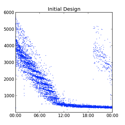
There are, however, significant problems with this approach. The most significant issue is that as you add data into the hourly and monthly fields, the document grows. Although MongoDB will pad the space allocated to documents, it must still reallocate these documents multiple times throughout the day, which degrades performance, as shown in Figure 4-2.

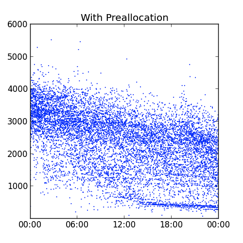
The solution to this problem lies in pre-allocating documents with fields holding 0 values before the documents are actually used. If the documents have all their fields fully populated at pre-allocation time, the documents never grow and never need to be moved. Another benefit is that MongoDB will not add as much padding to the documents, leading to a more compact data representation and better memory and disk utilization.

Figure 4-2. Performance with growing documents

One problem with our approach here, however, is that as we get toward the end of the day, the updates still become more expensive for MongoDB to perform, as shown in Figure 4-3. This is because MongoDB’s internal representation of our minute property is actually an array of key-value pairs that it must scan sequentially to find the minute slot we’re actually updating. So for the final minute of the day, MongoDB needs to examine 1,439 slots before actually finding the correct one to update. The solution to this is to build hierarchy into the minute property.

Figure 4-3. Performance with pre-allocated documents

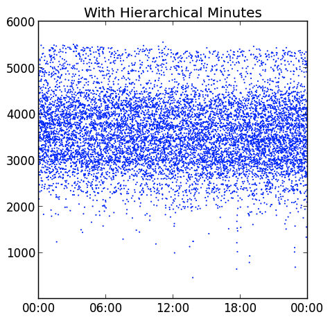
One document per page per day, hierarchical documents

To optimize update and insert operations, we’ll introduce some intra-document hierarchy. In particular, we’ll split the minute field into 24 hourly fields:

{
    _id: "20101010/site-1/apache_pb.gif",
    metadata: {
        date: ISODate("2000-10-10T00:00:00Z"),
        site: "site-1",
        page: "/apache_pb.gif" },
    daily: 5468426,
    hourly: {
        "0": 227850,
        "1": 210231,
        ...
        "23": 20457 },
    minute: {
        "0": {
            "0": 3612,
            "1": 3241,
            ...
            "59": 2130 },
        "1": {
        "60": ... ,
        },
        ...
        "23": {
            ...
            "1439": 2819 }
    }
}

This allows MongoDB to “skip forward” throughout the day when updating the minute data, which makes the update performance more uniform and faster later in the day, as shown in Figure 4-4.

Figure 4-4. Performance with hierarchical documents

Separate documents by granularity level

Pre-allocation of documents helps our update speed significantly, but we still have a problem when querying data for long, multiday periods like months or quarters. In such cases, storing daily aggregates in a higher-level document can speed up these queries.

This introduces a second set of upsert operations to the data collection and aggregation portion of your application, but the gains in reduction of disk seeks on the queries should be worth the costs. Consider the example schema presented in Example 4-1 and Example 4-2.

Example 4-1. Daily statistics

{
    _id: "20101010/site-1/apache_pb.gif",
    metadata: {
        date: ISODate("2000-10-10T00:00:00Z"),
        site: "site-1",
        page: "/apache_pb.gif" },
    hourly: {
        "0": 227850,
        "1": 210231,
        ...
        "23": 20457 },
    minute: {
        "0": {
            "0": 3612,
            "1": 3241,
            ...
            "59": 2130 },
        "1": {
            "0": ...,
        },
        ...
        "23": {
            "59": 2819 }
    }
}

Example 4-2. Monthly statistics

{
    _id: "201010/site-1/apache_pb.gif",
    metadata: {
        date: ISODate("2000-10-00T00:00:00Z"),
        site: "site-1",
        page: "/apache_pb.gif" },
    daily: {
        "1": 5445326,
        "2": 5214121,
        ... }
}

To support this operation, our event logging operation adds a second update operation, which does slow down the operation, but the gains in query performance should be well worth it.

Operations

This section outlines a number of common operations for building and interacting with real-time analytics-reporting systems. The major challenge is in balancing read and write performance. All our examples here use the Python programming language and the pymongo driver, but you can implement this system using any language you choose.

Log an event

Logging an event such as a page request (i.e., “hit”) is the main “write” activity for your system. To maximize performance, you’ll be doing in-place updates with the upsert=True to create documents if they haven’t been created yet. Consider the following example:

from datetime import datetime, time

def log_hit(db, dt_utc, site, page):

    # Update daily stats doc
    id_daily = dt_utc.strftime('%Y%m%d/') + site + page
    hour = dt_utc.hour
    minute = dt_utc.minute

    # Get a datetime that only includes date info
    d = datetime.combine(dt_utc.date(), time.min)
    query = {
        '_id': id_daily,
        'metadata': { 'date': d, 'site': site, 'page': page } }
    update = { '$inc': {
            'hourly.%d' % (hour,): 1,
            'minute.%d.%d' % (hour,minute): 1 } }
    db.stats.daily.update(query, update, upsert=True)

    # Update monthly stats document
    id_monthly = dt_utc.strftime('%Y%m/') + site + page
    day_of_month = dt_utc.day
    query = {
        '_id': id_monthly,
        'metadata': {
            'date': d.replace(day=1),
            'site': site,
            'page': page } }
    update = { '$inc': {
            'daily.%d' % day_of_month: 1} }
    db.stats.monthly.update(query, update, upsert=True)

The upsert operation (i.e., upsert=True) performs an update if the document exists, and an insert if the document does not exist.

Note

If, for some reason, you need to determine whether an upsert was an insert or an update, you can always check the result of the update operation:

>>> result = db.foo.update({'x': 15}, {'$set': {'y': 5} }, upsert=True)
>>> result['updatedExisting']
False
>>> result = db.foo.update({'x': 15}, {'$set': {'y': 6} }, upsert=True)
>>> result['updatedExisting']
True

Pre-allocate

To prevent document growth, we’ll pre-allocate new documents before the system needs them. In pre-allocation, we set all values to 0 so that documents don’t need to grow to accommodate updates. Consider the following function:

def preallocate(db, dt_utc, site, page):

    # Get id values
    id_daily = dt_utc.strftime('%Y%m%d/') + site + page
    id_monthly = dt_utc.strftime('%Y%m/') + site + page

    # Get daily metadata
    daily_metadata = {
        'date': datetime.combine(dt_utc.date(), time.min),
        'site': site,
        'page': page }
    # Get monthly metadata
    monthly_metadata = {
        'date': daily_m['d'].replace(day=1),
        'site': site,
        'page': page }

    # Initial zeros for statistics
    daily_zeros = [
        ('hourly.%d' % h, 0) for i in range(24) ]
    daily_zeros += [
        ('minute.%d.%d' % (h,m), 0)
        for h in range(24)
        for m in range(60) ]
    monthly_zeros = [
        ('daily.%d' % d, 0) for d in range(1,32) ]

    # Perform upserts, setting metadata
    db.stats.daily.update(
        {
            '_id': id_daily,
            'metadata': daily_metadata
        },
        { '$inc': dict(daily_zeros) },
        upsert=True)
    db.stats.monthly.update(
        {
            '_id': id_monthly,
            'daily': daily },
        { '$inc': dict(monthly_zeros) },
        upsert=True)

This function pre-allocates both the monthly and daily documents at the same time. The performance benefits from separating these operations are negligible, so it’s reasonable to keep both operations in the same function.

The question now arises as to when to pre-allocate the documents. Obviously, for best performance, they need to be pre-allocated before they are used (although the upsert code will actually work correctly even if it executes against a document that already exists). While we could pre-allocate the documents all at once, this leads to poor performance during the pre-allocation time. A better solution is to pre-allocate the documents probabilistically each time we log a hit:

from random import random
from datetime import datetime, timedelta, time

# Example probability based on 500k hits per day per page
prob_preallocate = 1.0 / 500000

def log_hit(db, dt_utc, site, page):
    if random.random() < prob_preallocate:
        preallocate(db, dt_utc + timedelta(days=1), site_page)
    # Update daily stats doc
    ...

Using this method, there will be a high probability that each document will already exist before your application needs to issue update operations. You’ll also be able to prevent a regular spike in activity for pre-allocation, and be able to eliminate document growth.

Retrieving data for a real-time chart

This example describes fetching the data from the above MongoDB system for use in generating a chart that displays the number of hits to a particular resource over the last hour.

We can use the following query in a find_one operation at the Python console to retrieve the number of hits to a specific resource (i.e., /index.html) with minute-level granularity:

>>> db.stats.daily.find_one(
...     {'metadata': {'date':dt, 'site':'site-1', 'page':'/index.html'}},
...     { 'minute': 1 })

Alternatively, we can use the following query to retrieve the number of hits to a resource over the last day, with hour-level granularity:

code,sourceCode,pycon
>>> db.stats.daily.find_one(
...     {'metadata': {'date':dt, 'site':'site-1', 'page':'/foo.gif'}},
...     { 'hourly': 1 })

If we want a few days of hourly data, we can use a query in the following form:

>>> db.stats.daily.find(
...     {
...         'metadata.date': { '$gte': dt1, '$lte': dt2 },
...         'metadata.site': 'site-1',
...         'metadata.page': '/index.html'},
...     { 'metadata.date': 1, 'hourly': 1 } },
...     sort=[('metadata.date', 1)])

To support these query operations, we need to create a compound index on the following daily statistics fields: metadata.site, metadata.page, and metadata.date, in that order. This is because our queries have equality constraints on site and page, and a range query on date. To create the appropriate index, we can execute the following code:

>>> db.stats.daily.ensure_index([
...     ('metadata.site', 1),
...     ('metadata.page', 1),
...     ('metadata.date', 1)])

Get data for a historical chart

To retrieve daily data for a single month, we can use the following query:

>>> db.stats.monthly.find_one(
...     {'metadata':
...         {'date':dt,
...         'site': 'site-1',
...         'page':'/index.html'}},
...     { 'daily': 1 })

To retrieve several months of daily data, we can use a variation of the preceding query:

>>> db.stats.monthly.find(
...     {
...         'metadata.date': { '$gte': dt1, '$lte': dt2 },
...         'metadata.site': 'site-1',
...         'metadata.page': '/index.html'},
...     { 'metadata.date': 1, 'hourly': 1 } },
...     sort=[('metadata.date', 1)])

To execute these queries efficiently, we need an index on the monthly aggregate similar to the one we used for the daily aggregate:

>>> db.stats.monthly.ensure_index([
...     ('metadata.site', 1),
...     ('metadata.page', 1),
...     ('metadata.date', 1)])

This field order will efficiently support range queries for a single page over several months.

Sharding Concerns

Although the system as designed can support quite a large read and write load on a single-master deployment, sharding can further improve your performance and scalability. Your choice of shard key may depend on the precise workload of your deployment, but the choice of site-page is likely to perform well and lead to a well balanced cluster for most deployments.

To enable sharding for the daily and statistics collections, we can execute the following commands in the Python console:

>>> db.command('shardcollection', 'dbname.stats.daily', {
    ...     key : { 'metadata.site': 1, 'metadata.page' : 1 } })
{ "collectionsharded" : "dbname.stats.daily", "ok" : 1 }
>>> db.command('shardcollection', 'dbname.stats.monthly', {
...     key : { 'metadata.site': 1, 'metadata.page' : 1 } })
{ "collectionsharded" : "dbname.stats.monthly", "ok" : 1 }

One downside of the { metadata.site: 1, metadata.page: 1 } shard key is that if one page dominates all your traffic, all updates to that page will go to a single shard. This is basically unavoidable, since all updates for a single page are going to a single document.

You may wish to include the date in addition to the site and page fields so that MongoDB can split histories and serve different historical ranges with different shards. Note that this still does not solve the problem; all updates to a page will still go to one chunk, but historical queries will scale better.

To enable the three-part shard key, we just update our shardcollection with the new key:

>>> db.command('shardcollection', 'dbname.stats.daily', {
    ...     'key':{'metadata.site':1,'metadata.page':1,'metadata.date':1}})
{ "collectionsharded" : "dbname.stats.daily", "ok" : 1 }
>>> db.command('shardcollection', 'dbname.stats.monthly', {
...     'key':{'metadata.site':1,'metadata.page':1,'metadata.date':1}})
{ "collectionsharded" : "dbname.stats.monthly", "ok" : 1 }

Hierarchical Aggregation

Although the techniques of Pre-Aggregated Reports can satisfy many operational intelligence system needs, it’s often desirable to calculate statistics at multiple levels of abstraction. This section describes how we can use MongoDB’s mapreduce command to convert transactional data to statistics at multiple layers of abstraction.

For clarity, this case study assumes that the incoming event data resides in a collection named events. This fits in well with Storing Log Data, making these two techniques work well together.

Solution Overview

The first step in the aggregation process is to aggregate event data into statistics at the finest required granularity. Then we’ll use this aggregate data to generate the next least specific level granularity and repeat this process until we’ve generated all required views.

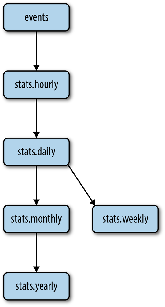
This solution uses several collections: the raw data (i.e., events) collection as well as collections for aggregated hourly, daily, weekly, monthly, and yearly statistics. All aggregations use the mapreduce database command in a hierarchical process. Figure 4-5 illustrates the input and output of each job.

Figure 4-5. Hierarchical aggregation

Schema Design

When designing the schema for event storage, it’s important to track the events included in the aggregation and events that are not yet included.

If you can batch your inserts into the events collection, you can use an autoincrement primary key by using the find_and_modify command to generate the _id values, as shown here:

>>> obj = db.my_sequence.find_and_modify(
...     query={'_id':0},
...     update={'$inc': {'inc': 50}}
...     upsert=True,
...     new=True)
>>> batch_of_ids = range(obj['inc']-50, obj['inc'])

However, in many cases you can simply include a timestamp with each event that you can use to distinguish processed events from unprocessed events.

This example assumes that you are calculating average session length for logged-in users on a website. The events will have the following form:

{
    "userid": "rick",
    "ts": ISODate('2010-10-10T14:17:22Z'),
    "length":95
}

The operations described here will calculate total and average session times for each user at the hour, day, week, month, and year. For each aggregation, we’ll store the number of sessions so that MongoDB can incrementally recompute the average session times. The aggregate document will resemble the following:

{
   _id: { u: "rick", d: ISODate("2010-10-10T14:00:00Z") },
   value: {
       ts: ISODate('2010-10-10T15:01:00Z'),
       total: 254,
       count: 10,
       mean: 25.4 }
}

MapReduce

The MapReduce algorithm and its MongoDB implementation, the mapreduce command, is a popular way to process large amounts of data in bulk. If you’re not familiar with MapReduce, the basics are illustrated in the following pseudocode:

from collections import defaultdict
def map_reduce(input, output, query, mapf, reducef, finalizef):
    # Map phase
    map_output = []
    for doc in input.find(output):
        map_output += mapf(doc) 

    # Shuffle phase
    map_output.sort() 
    docs_by_key = groupby_keys(map_output)

    # Reduce phase
    reduce_output = []
    for key, values in docs_by_key:
        reduce_output.append({
            '_id': key,
            'value': reducef(key, values) })

    # Finalize phase
    finalize_output = [] 
    for doc in reduce_output:
        key, value = doc['_id'], doc['value']
        reduce_output[key] = finalizef(key, value)

    output.remove() 
    output.insert(finalize_output)

In MongoDB, mapf actually calls an emit function to generate zero or more documents to feed into the next phase. The signature of the mapf function is also modified to take no arguments, passing the document in the this JavaScript keyword.

Sorting is not technically required; the purpose is to group documents with the same key together. Sorting is just one way to do this.

Finalize is not required, but can be useful for computing things like mean values given a count and sum computed by the other parts of MapReduce.

MongoDB provides several different options of how to store your output data. In this code, we’re mimicking the output mode of replace.

The nice thing about this algorithm is that each of the phases can be run in parallel. In MongoDB, this benefit is somewhat limited by the presence, as of version 2.2, of a global JavaScript interpreter lock that forces all JavaScript in a single MongoDB process to run serially. Sharding allows you to get back some of this performance, but the full benefits of MapReduce still await the removal of the JavaScript lock from MongoDB.

Operations

This section assumes that all events exist in the events collection and have a timestamp. The operations are to aggregate from the events collection into the smallest aggregate—hourly totals—and then aggregate from the hourly totals into coarser granularity levels. In all cases, these operations will store aggregation time as a last_run variable.

Creating hourly views from event collections

To do our lowest-level aggregation, we need to first create a map function, as shown here:

mapf_hour = bson.Code('''function() {
    var key = {
        u: this.userid,
        d: new Date(
            this.ts.getFullYear(),
            this.ts.getMonth(),
            this.ts.getDate(),
            this.ts.getHours(),
            0, 0, 0);
    emit(
        key,
        {
            total: this.length,
            count: 1,
            mean: 0,
            ts: null });
}''')

In this case, mapf_hour emits key-value pairs that contain the data you want to aggregate, as you’d expect. The function also emits a ts value that makes it possible to cascade aggregations to coarser-grained aggregations (hour to day, etc.).

Next, we define the following reduce function:

reducef = bson.Code('''function(key, values) {
    var r = { total: 0, count: 0, mean: 0, ts: null };
    values.forEach(function(v) {
        r.total += v.total;
        r.count += v.count;
    });
    return r;
}''')

The reduce function returns a document in the same format as the output of the map function. This pattern for map and reduce functions makes MapReduce processes easier to test and debug.

While the reduce function ignores the mean and ts (timestamp) values, the finalize step, as follows, computes these data:

finalizef = bson.Code('''function(key, value) {
    if(value.count > 0) {
       value.mean = value.total / value.count;
    }
    value.ts = new Date();
    return value;
}''')

With the preceding functions defined, our actual mapreduce call resembles the following:

cutoff = datetime.utcnow() - timedelta(seconds=60)
query = { 'ts': { '$gt': last_run, '$lt': cutoff } }

db.events.map_reduce(
    map=mapf_hour,
    reduce=reducef,
    finalize=finalizef,
    query=query,
    out={ 'reduce': 'stats.hourly' })

last_run = cutoff

Output Modes

Here, we’re using the 'reduce' output mode. MongoDB’s mapreduce provides several of these modes for different use cases:

replace

In this mode, MongoDB will drop any collection that currently exists with the output name before writing the mapreduce results into it.

merge

In this mode, MongoDB does not drop the output collection first, but will overwrite any existing results with the same key with the results of the mapreduce results.

reduce

In this mode, MongoDB treats the output collection as additional input to the reduce phase. This mode is most useful for incremental aggregation, where we wish to refine existing results based on new data.

inline

In this mode, no output collection is written; the results are returned as the result of the mapreduce command itself.

The cutoff variable allows you to process all events that have occurred since the last run but before one minute ago. This allows for some delay in logging events. You can safely run this aggregation as often as you like, provided that you update the last_run variable each time.

Since we’ll be repeatedly querying the events collection by date, it’s important to maintain an index on this property:

>>> db.events.ensure_index('ts')

Deriving day-level data

To calculate daily statistics, we can use the hourly statistics as input. We’ll begin with the following map function:

mapf_day = bson.Code('''function() {
    var key = {
        u: this._id.u,
        d: new Date(
            this._id.d.getFullYear(),
            this._id.d.getMonth(),
            this._id.d.getDate(),
            0, 0, 0, 0) };
    emit(
        key,
        {
            total: this.value.total,
            count: this.value.count,
            mean: 0,
            ts: null });
}''')

The map function for deriving day-level data differs from this initial aggregation in the following ways:

• The aggregation key is the userid-date rather than userid-hour to support daily aggregation.
• The keys and values emitted (i.e., emit()) are actually the total and count values from the hourly aggregates, rather than properties from event documents.

This is the case for all the higher-level aggregation operations. Because the output of this map function is the same as the previous map function, we can actually use the same reduce and finalize functions. The actual code driving this level of aggregation is as follows:

cutoff = datetime.utcnow() - timedelta(seconds=60)
query = { 'value.ts': { '$gt': last_run, '$lt': cutoff } }

db.stats.hourly.map_reduce(
    map=mapf_day,
    reduce=reducef,
    finalize=finalizef,
    query=query,
    out={ 'reduce': 'stats.daily' })

last_run = cutoff

There are a couple of things to note here. First of all, the query is not on ts now, but value.ts, the timestamp written during the finalization of the hourly aggregates. Also note that we are, in fact, aggregating from the stats.hourly collection into the stats.daily collection.

Because we’ll be running this query on a regular basis, and the query depends on the value.ts field, we’ll want to create an index on value.ts:

>>> db.stats.hourly.ensure_index('value.ts')

Weekly and monthly aggregation

We can use the aggregated day-level data to generate weekly and monthly statistics. A map function for generating weekly data follows:

mapf_week = bson.Code('''function() {
    var key = {
        u: this._id.u,
        d: new Date(
            this._id.d.valueOf()
            - dt.getDay()*24*60*60*1000) };
    emit(
        key,
        {
            total: this.value.total,
            count: this.value.count,
            mean: 0,
            ts: null });
}''')

Here, to get the group key, the function takes the current day and subtracts days until you get the beginning of the week. In the monthly map function, we’ll use the first day of the month as the group key, as follows:

mapf_month = bson.Code('''function() {
        d: new Date(
            this._id.d.getFullYear(),
            this._id.d.getMonth(),
            1, 0, 0, 0, 0) };
    emit(
        key,
        {
            total: this.value.total,
            count: this.value.count,
            mean: 0,
            ts: null });
}''')

These map functions are identical to each other except for the date calculation.

To make our aggregation at these levels efficient, we need to create indexes on the value.ts field in each collection that serves as input to an aggregation:

>>> db.stats.daily.ensure_index('value.ts')
>>> db.stats.monthly.ensure_index('value.ts')

Refactor map functions

Using Python’s string interpolation, we can refactor the map function definitions as follows:

mapf_hierarchical = '''function() {
    var key = {
        u: this._id.u,
        d: %s };
    emit(
        key,
        {
            total: this.value.total,
            count: this.value.count,
            mean: 0,
            ts: null });
}'''

mapf_day = bson.Code(
    mapf_hierarchical % '''new Date(
            this._id.d.getFullYear(),
            this._id.d.getMonth(),
            this._id.d.getDate(),
            0, 0, 0, 0)''')

mapf_week = bson.Code(
    mapf_hierarchical % '''new Date(
            this._id.d.valueOf()
            - dt.getDay()*24*60*60*1000)''')

mapf_month = bson.Code(
    mapf_hierarchical % '''new Date(
            this._id.d.getFullYear(),
            this._id.d.getMonth(),
            1, 0, 0, 0, 0)''')

mapf_year = bson.Code(
    mapf_hierarchical % '''new Date(
            this._id.d.getFullYear(),
            1, 1, 0, 0, 0, 0)''')

Now, we’ll create an h_aggregate function to wrap the map_reduce operation to reduce code duplication:

def h_aggregate(icollection, ocollection, mapf, cutoff, last_run):
     query = { 'value.ts': { '$gt': last_run, '$lt': cutoff } }
     icollection.map_reduce(
         map=mapf,
         reduce=reducef,
         finalize=finalizef,
         query=query,
         out={ 'reduce': ocollection.name })

With h_aggregate defined, we can perform all aggregation operations as follows:

cutoff = datetime.utcnow() - timedelta(seconds=60)

# First step is still special
query = { 'ts': { '$gt': last_run, '$lt': cutoff } }
db.events.map_reduce(
    map=mapf_hour, reduce=reducef,
    finalize=finalizef, query=query,
    out={ 'reduce': 'stats.hourly' })

# But the other ones are not
h_aggregate(db.stats.hourly, db.stats.daily, mapf_day, cutoff, last_run)
h_aggregate(db.stats.daily, db.stats.weekly, mapf_week, cutoff, last_run)
h_aggregate(db.stats.daily, db.stats.monthly, mapf_month, cutoff, last_run)
h_aggregate(db.stats.monthly, db.stats.yearly, mapf_year, cutoff, last_run)

last_run = cutoff

As long as we save and restore the last_run variable between aggregations, we can run these aggregations as often as we like, since each aggregation operation is incremental (i.e., using output mode 'reduce').

Sharding Concerns

When sharding, we need to ensure that we don’t choose the incoming timestamp as a shard key, but rather something that varies significantly in the most recent documents. In the previous example, we might consider using the userid as the most significant part of the shard key.

To prevent a single, active user from creating a large chunk that MongoDB cannot split, we’ll use a compound shard key with username-timestamp on the events collection as follows:

>>> db.command('shardcollection','dbname.events', {
... 'key' : { 'userid': 1, 'ts' : 1} } )
{ "collectionsharded": "dbname.events", "ok" : 1 }

To shard the aggregated collections, we must use the _id field to work well with mapreduce, so we’ll issue the following group of shard operations in the shell:

>>> db.command('shardcollection', 'dbname.stats.daily', {
...      'key': { '_id': 1 } })
{ "collectionsharded": "dbname.stats.daily", "ok" : 1 }
>>> db.command('shardcollection', 'dbname.stats.weekly', {
...      'key': { '_id': 1 } })
{ "collectionsharded": "dbname.stats.weekly", "ok" : 1 }
>>> db.command('shardcollection', 'dbname.stats.monthly', {
...      'key': { '_id': 1 } })
{ "collectionsharded": "dbname.stats.monthly", "ok" : 1 }
>>> db.command('shardcollection', 'dbname.stats.yearly', {
...      'key': { '_id': 1 } })
{ "collectionsharded": "dbname.stats.yearly", "ok" : 1 }

We also need to update the h_aggregate MapReduce wrapper to support sharded output by adding 'sharded':True to the out argument. Our new h_aggregate now looks like this:

def h_aggregate(icollection, ocollection, mapf, cutoff, last_run):
     query = { 'value.ts': { '$gt': last_run, '$lt': cutoff } }
     icollection.map_reduce(
         map=mapf,
         reduce=reducef,
         finalize=finalizef,
         query=query,
         out={ 'reduce': ocollection.name, 'sharded': True })