I love reading popular science, a hobby that stems from a happy childhood encounter with Isaac Asimov’s “science fact” books after I’d consumed all of his science fiction ones in the local library. I was a voracious reader, and soon my interests spilled over to other types of books, such as Martin Gardner’s mathematics books and Stephen Jay Gould’s biology books. While I didn’t necessarily fully understand the science behind them all, the material was fascinating enough for me to develop a lifelong passion for such writing.
Nestled among my science books is a particular genre of popular writing that equally and frequently brought me wonder and amazement—popular economics books. No doubt the first book that probably flashed through your mind is the immensely popular and widely read Freakonomics (William Morrow). While that’s a great book, the one book on popular economics that always tops my list (and I readily admit it might be entirely due to the mental image I get when I think of the title) is the Armchair Economist by Stephen E. Landsburg (Free Press).
Something from the Armchair Economist that stuck in my mind for a long time, eventually blossoming into this book, is how Landsburg described economics:
Economics is…about observing the world with genuine curiosity and admitting that it is full of mysteries....Sometimes the mysteries themselves…are hard to solve, so we practice by trying to solve similar mysteries in fictional worlds that we invent and call models.
In this chapter, we explore how to model some very basic economic theories and then investigate how they work.
Economists sometimes ask a rhetorical and seemingly silly question: “Who feeds Paris?”[9] The Parisians themselves, of course; who else? However, neither the question nor the answer is straightforward. There is a lot more to it than meets the eye.
During the days of the Soviet Union and the Cold War, the story goes, a Soviet official visited the United States and went into a supermarket. The brightly lit aisles were filled with all kinds of products from peanut butter to gardening tools. “Very impressive,” said the official. “But how can you make sure that all the supermarkets have all these items?”
While we might laugh at the official’s lack of understanding of market economy, you can probably find a parallel in the question of who feeds Paris. You’ve probably never heard of the Parisian sidewalk cafes running out of coffee, so how do they know what kind of coffee, and how much, to stock? How do the fashion boutiques know which clothes to stock and how much to sell them for? How does Darty (a French electronics chain) know which are the best mobile phones to sell?
These questions are answered succinctly by 18th-century Scottish economist and social philosopher Adam Smith. His book An Inquiry into the Nature and Causes of the Wealth of Nations (excerpted here) is considered the first modern work of economics, while he himself is often regarded as the father of economics:
It is not from the benevolence of the butcher, the brewer or the baker, that we expect our dinner, but from their regard to their own interest. We address ourselves, not to their humanity but to their self-love, and never talk to them of our own necessities but of their advantages.
Smith coined the metaphor of the “invisible hand” to label this natural inclination, effectively describing what we know today as the market economy. In this chapter, we will simulate a market economy to see if we can observe the invisible hand in action.
First, let’s take stock of the different roles and features of an ideal market economy (which are what we want to simulate).
- Producers
The people who produce the goods. Producers create the goods and sell them to the consumers at a price.
- Consumers
The people who consume the goods created by the producers. Consumers buy goods from producers at a price.
- Price
This is the value at which producers agree to exchange goods with consumers. The price is set by each producer.
- Supply
The amount of goods generated by the producers.
- Demand
The amount of goods that the consumers want to buy.
- Market
The overall ecosystem of buying and selling goods from and to producers and consumers.
In this idealized market economy, we will have the producers creating goods and selling them to consumers for a price. Each producer sets his own price.
The consumers, in turn, buy goods from the producer. However, this happens only if the consumer thinks the price is reasonable. Consumers have a certain amount of demand and will buy to fulfill that demand. In addition, consumers can buy from any producer, and will buy from the producer who sells at the cheapest price first.
We start off our exercise with the producer. The Producer class is a rather simple one, as
shown in Example 4-1.
Example 4-1. Producer class
class Producer
  attr_accessor :supply, :price
  def initialize
    @supply, @price = 0, 0
  end

  def generate_goods
   @supply += SUPPLY_INCREMENT if @price > COST
  end

  def produce
    if @supply > 0
      @price *= PRICE_DECREMENT unless @price < COST
    else
      @price *= PRICE_INCREMENT
      generate_goods
    end
  end
end
Producer has two variables:
supply, which is the amount of unsold goods that the
producer has at that moment, and price, which is the
price she wants to sell the goods for. Both are initialized to 0 when
the Producer class is first
instantiated.
The Producer class also has a
produce method that, well, produces the goods and
sets the price:
def produce
  if @supply > 0
    @price *= PRICE_DECREMENT unless @price < COST
  else
    @price *= PRICE_INCREMENT
    generate_goods
  end
end
While the price is presumably set immediately after instantiation,
we want to change the price accordingly to be more competitive with the
other producers in the same market. To do this, we multiply the current
price with either a PRICE_DECREMENT or
PRICE_INCREMENT multiplier. Whether to increase or
reduce the price depends on how well the goods have sold in the
past.
If all the goods have been sold, this means they were well
received, so the producer will want to make more—by calling the
generate_goods method—and also increase the price
slightly, to generate more profit.
If that’s not the case, and there are still unsold goods, the
producer will want to make them more attractive by dropping the price a
little. Naturally, she will not decrease the price if it’s below the
cost of generating the goods, indicated by the constant
COST.
The Producer class also has an
instance method, generate_goods, which will create
the goods. As mentioned earlier, this is called only if the producer’s
supply runs out:
def generate_goods
 @supply += SUPPLY_INCREMENT if Market.average_price > COST
end
The generate_goods method increases the amount of
goods by adding on to its current supply a
SUPPLY_INCREMENT amount. Of course, this happens only
if the price is more than the cost of generating the goods.
Next is the consumer. The Consumer class, shown in Example 4-2, is an even simpler beast. It has only one purpose:
to consume the goods up to the level of its demand.
Example 4-2. Consumer class
class Consumer
  attr_accessor :demands

  def initialize
    @demands = 0
  end

  def buy
    until @demands <= 0 or Market.supply <= 0
      cheapest_producer = Market.cheapest_producer
      if cheapest_producer
        @demands *= 0.5 if cheapest_producer.price > MAX_ACCEPTABLE_PRICE
        cheapest_supply = cheapest_producer.supply
        if @demands > cheapest_supply
          @demands -= cheapest_supply
          cheapest_producer.supply = 0
        else
          cheapest_producer.supply -= @demands
          @demands = 0
        end
      end
    end
  end
end
The Consumer class has a single
variable, demands, which indicates the amount of
goods it requires to fulfill its needs. The main method for the Consumer class is buy. When
the buy method is called, the consumer will continue
to buy goods until his demand is met or the supply in the whole market
runs out.
Each consumer first looks for the cheapest producer and buys as much as it can from her. When the consumer buys from the producer, the producer’s supply decreases and the demand also decreases accordingly. If the supplies run out first, the consumer buys from the next producer until his demand is satiated.
However, the consumer is not a buying machine. If the cheapest
price is higher than the maximum acceptable price set by the constant
MAX_ACCEPTABLE_PRICE, the consumer’s demand is
reduced by half.
Before we get into the simulation script, we’re going to create
some convenience methods. We’ll define all of these convenience methods
as static methods in a Market class, as shown
in Example 4-3.
Example 4-3. Market class
class Market
  def self.average_price
    ($producers.inject(0.0) { |memo, producer| memo + producer.price}/
                              $producers.size).round(2)
  end

  def self.supply
    $producers.inject(0) { |memo, producer| memo + producer.supply }
  end

  def self.demand
    $consumers.inject(0) { |memo, consumer| memo + consumer.demands }
  end

  def self.cheapest_producer
    producers = $producers.find_all {|f| f.supply > 0}
    producers.min_by{|f| f.price}
  end
end
The first of these convenience methods is
average_price. We will be using this method to get
the average price of the goods based on the prices from all the
producers. Next are the supply and demand
methods, which return the collective amounts of goods and demands of all
the producers and all the consumers, respectively. Finally, we have a
cheapest_producer method, which returns the cheapest
producer. We determine this by finding all the producers who still have
goods, comparing them by price, and returning the one with the
cheapest price.
Now that we have all the pieces in place, let’s get to the simulation. To prepare for it, we need to first create the population of producers and consumers, as shown in Example 4-4.
Example 4-4. Populating the simulation
$producers = []
NUM_OF_PRODUCERS.times do
  producer = Producer.new
  producer.price = COST + rand(MAX_STARTING_PROFIT)
  producer.supply = rand(MAX_STARTING_SUPPLY)
  $producers << producer
end

$consumers = []
NUM_OF_CONSUMERS.times do
  $consumers << Consumer.new
end

$generated_demand  = []
SIMULATION_DURATION.times {|n| $generated_demand << ((Math.sin(n)+2)*20).round  }
We store the producers in the global array
$producers and the consumers in the global array
$consumers. Each producer is created with a randomly
generated price that is higher than the cost of producing the goods
(COST), as well as a randomly generated amount of goods. We
don’t do anything to the consumers that are created at this point; we’ll
get to them in the simulation loop later.
We’ll also create a fluctuating
generated demand and store that in the
$generated_demand variable. This will be used during
the simulation to represent the fluctuation of demand over a period of
time. This generated demand roughly follows a sine wave.
The simulation loop is shown in Example 4-5. Before
we actually go into the loop, we prepare two empty arrays:
demand_supply and price_demand.
These are used to store the values generated from the simulation. The
names of each array indicate what it contains; the
demand_supply array stores the changes of demand
versus supply of goods over the simulation period, while the
price_demand array stores the changes of price versus
demand over the same period.
Example 4-5. Simulation loop
SIMULATION_DURATION.times do |t|
  $consumers.each do |consumer|
    consumer.demands = $generated_demand[t]
  end
  demand_supply << [t, Market.demand, Market.supply]

  $producers.each do |producer|
    producer.produce
  end

  price_demand << [t, Market.average_price, Market.demand]

  until Market.demand == 0 or Market.supply == 0 do
    $consumers.each do |consumer|
      consumer.buy
    end
  end
end

write("demand_supply", demand_supply)
write("price_demand", price_demand)
The simulation is a loop that runs
SIMULATION_DURATION times and executes a series of
producer and consumer actions.
At the start of the loop, we set every consumer’s demand to be a
point in the demand curve in $generated_demand.
Before we start with the producer, we populate the
demand_supply array with the current market demand
and supply. Then we loop through each producer and get her to create and
set the price of goods by calling the produce method.
This randomly generates the price of goods for each producer.
After that and before looping through each
consumer, we populate the price_demand array
with the average price of goods and the market demand. Finally, we loop
through each consumer and get him to buy. We add in an extra loop to
make sure all the demands are met unless the supply of goods runs out
first. With this, we end a single simulation loop.
At the end of SIMULATION_DURATION loops,
we use the write method to write the data to a CSV
file, which we will use to analyze our simulation next (see Example 4-6).
Example 4-6. The write method
def write(name,data)
  CSV.open("#{name}.csv", 'w') do |csv|
    data.each do |row|
      csv << row
    end
  end
end
The write method simply uses the CSV
library built into Ruby 1.9 and creates a file for writing, then loops
through the given data array, writing each item of the array as a line
in the CSV file.
Last, before we run the simulation to generate the files, let’s look at the constants that we referred to in the simulation but whose values we never really examined (Example 4-7). This is not exactly exciting new stuff, but it will help us understand the values of the analysis later on.
Example 4-7. Constants used in the simulation
SIMULATION_DURATION = 150
NUM_OF_PRODUCERS = 10
NUM_OF_CONSUMERS = 10

MAX_STARTING_SUPPLY = 20
SUPPLY_INCREMENT = 80

COST = 5
MAX_ACCEPTABLE_PRICE = COST * 10
MAX_STARTING_PROFIT = 5
PRICE_INCREMENT = 1.1
PRICE_DECREMENT = 0.9
In Example 4-7, you can see that we will be running the simulation for 150 ticks with 10 producers and 10 consumers. The starting supply for the producers is somewhere between 0 and 20, while at each tick, depending on whether the supply runs out in the previous tick or not, each producer creates 80 units of goods at a cost of $5 each.
For the consumer, the maximum acceptable price of the goods is a multiple of the cost of the goods; for the producer, the starting profits are not more than $5 above the cost. Finally, the price of the goods increases or decreases by 10% each tick.
Now we can finally run the simulation, which should finish quite quickly. You should end up with two files, demand_supply.csv and price_demand.csv. We’ll be using these two files in the next section when we inspect the results of our simulation.
As in Chapter 3, we’ll be using R scripts to chart and analyze the patterns of the data we’ve just generated from our simulation. However, our approaches will differ slightly. In Chapter 3, we were investigating the results of a simulation, while here we are trying to simulate and re-enact an existing effect. In other words, we didn’t know the actual answers to the questions we were asking when we ran the Monte Carlo simulations in Chapter 3, but we do know what the results should be here.
Let’s take a look at the first data file we generated, demand_supply.csv. It has three columns; the first is a point in time, the second is the demand of the goods at that point in time, and the third is the supply of the goods at that time. We’ll grab this file, parse it, and generate two line charts—one superimposed on the other (see Example 4-8).
Example 4-8. Analyzing the demand and supply
library(ggplot2)
data <- read.table("demand_supply.csv", header=F, sep=",")

pdf("demand_supply.pdf")
ggplot(data = data) + scale_color_grey(name="Legend") +
  geom_line(aes(x  = V1, y = V2, color = "demand")) +
  geom_line(aes(x  = V1, y = V3, color = "supply")) +
  scale_y_continuous("amount") +
  scale_x_continuous("time")

dev.off()
As in Chapter 3, we use the
ggplot2 library first, then read in the data from the
CSV file. The three columns—time, demand, and supply—are automatically
labeled V1, V2, and V3. We use ggplot to create the
base data plot, then set the scale color to
grayscale. Next, we attach two
geom_lines that set the necessary x- and y-axes with
the correct data column. Finally, we add in the x- and y-axis
labels.
We predetermined the demand pattern, which should be almost a sine wave, though sharper since we rounded off the numbers (see Figure 4-1). What interests us is the supply pattern. If the basic theories of economics are right and we’ve coded the simulation correctly, then the supply of the goods should fall when the demand increases, and vice versa. If you look at Figure 4-1, you will see this same pattern, so it’s relief all around.
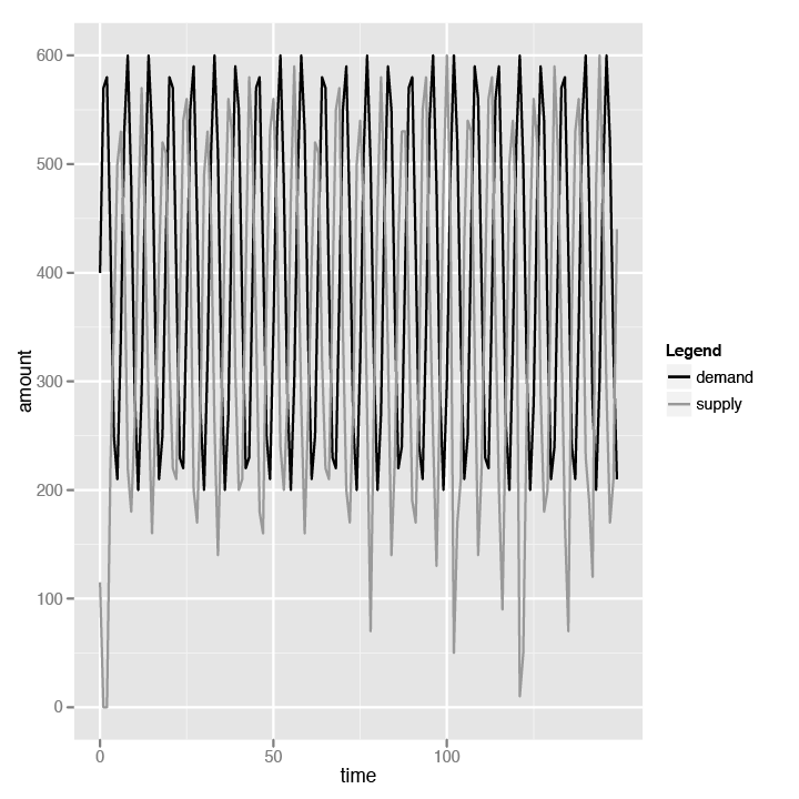
This might seem obvious, but if
you take a second look at the Producer and Consumer classes, you’ll see that neither the
produce nor the buy logic hinge on each other. The produce logic
generates more goods only if the supplies are all sold out. The producer
doesn’t produce to meet the demands of the consumer; she produces when
her own supplies run out.
Similarly, the buy logic chooses the cheapest goods and consumes until the demand is satiated (we added in the mechanism to stop when the supply in the market runs out, to prevent an infinite loop). The consumer doesn’t care about the supply of the goods; he cares only about the price of the goods and will consume until his demands are satisfied or the goods become too expensive.
Let’s take a look at the second data file, price_demand.csv. It has three columns again—the first is a point in time, the second is the average price of goods from all producers, and the third is the overall market demand. In Example 4-9, we do pretty much the same thing as in Example 4-8.
Example 4-9. Analyzing the price and demand
library(ggplot2)
data <- read.table("price_demand.csv", header=F, sep=",")

pdf("price_demand.pdf")
ggplot(data = data) + scale_color_grey(name="Legend") +
  geom_line(aes(x  = V1, y = V2, color = "price")) +
  geom_line(aes(x  = V1, y = log2(V3)-3, color = "demand")) +
    scale_y_continuous("amount") +
    scale_x_continuous("time")

dev.off()
There is a difference in charting the price, though. We take the logarithm of the demand to base 2 and chart that instead of the actual demand. Why do we do that? It’s because if we charted the actual demand value, we would not be able to see how the price relates to the demand, and vice versa, as the scale of the demand is much higher than that of the price.
We can make a couple of quick observations from the chart in Figure 4-2. First, we can see that the peak price of goods follows after the peak demand. Similarly, the price is lowest after the demand has fallen to its lowest.
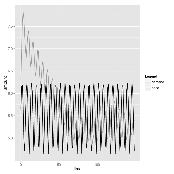
Second, while the price fluctuates with the demand, it actually
decreases over time until it stabilizes at a price between $5 and $5.50.
Notice this corresponds with the cost of creating goods, which we set at
$5 at the beginning of the simulation. The logic in the
Producer class’s produce
method prevents the price from ever dropping below the cost. This is the
reason why the price stabilizes at around $5. But why does the price
drop at all?
This is due to the market economy again. Remember that the consumer always buys the cheapest goods first. This means the producer with the higher prices will have unsold goods, which in turn forces the prices to go down. The end results are that the average price goes down until it nears the cost of producing the goods. Finally, we see the invisible hand! The invisible hand of Adam Smith has weighed in on our simulation and pushed the prices down.
Now that we have witnessed the invisible hand and charted its effects, let’s get slightly more complicated.
In the previous simulation, every producer creates only one type of
goods, which we imaginatively called goods. This, of
course, is not realistic (nothing modeled in economics is realistic, but
that’s a different point). In our next simulation, we will have producers
creating two types of goods. These producers are farmers who can rear
chickens or ducks on their farms. These farmers will rear either animal
depending on the profits they can get in return for it. There is no cost
to switching animals, and the farmers will remorselessly switch at a
slightest hint of a profit to be earned.
What we want to investigate is the relationship between the prices of ducks and chickens, as well as the relationship between the supply of ducks and chickens over time. Let’s look at changes we’ll need to make to our simulation.
We start off with the Producer class,
which as you might have guessed, has the most changes, as shown in Example 4-10.
Example 4-10. Producer class for second simulation
class Producer
  attr_accessor :supply, :price
  def initialize
    @supply, @supply[:chickens], @supply[:ducks] = {}, 0, 0
    @price, @price[:chickens], @price[:ducks] = {}, 0, 0
  end

  def change_pricing
    @price.each do |type, price|
      if @supply[type] > 0
        @price[type] *= PRICE_DECREMENT unless @price[type] < COST[type]
      else
        @price[type] *= PRICE_INCREMENT
      end
    end
  end

  def generate_goods
    to_produce = Market.average_price(:chickens) > Market.average_price(:ducks) ?
        :chickens : :ducks
    @supply[to_produce] += (SUPPLY_INCREMENT) if @price[to_produce] > COST[to_produce]
  end

  def produce
    change_pricing
    generate_goods
  end
end
The first change you’ll observe is that while we still have the
supply and price variables, they
are no longer integers but are in fact hashes, with the key being either
chickens or ducks. Next, the generate_goods method is
slightly different. The farmer will only produce either chickens or
ducks depending on the prices. If the average market price of duck is
higher, she’ll produce more ducks, and if the average market price of
chicken is higher, she’ll produce more chickens.
Notice that in Example 4-1 in the previous
simulation, the produce method changes the pricing,
then calls the generate_goods method to generate the
goods. In this simulation, the Producer class has a separate method named
changed_pricing that will iterate through the prices
of both chickens and ducks and check if there is any unsold poultry
left. If there is, the farmer will lower the price in the hope that it
can get sold more easily.
Finally, the produce method in this simulation
is a simple one that just calls change_pricing and
then generates the goods.
The changes to the Consumer
class, as shown in Example 4-11, are done in the same way
as the Producer class.
Example 4-11. Consumer class for the second simulation
class Consumer
  attr_accessor :demands

  def initialize
    @demands = 0
  end

  def buy(type)
    until @demands <= 0 or Market.supply(type) <= 0
      cheapest_producer = Market.cheapest_producer(type)
      if cheapest_producer
        @demands *= 0.5 if cheapest_producer.price[type] > MAX_ACCEPTABLE_PRICE[type]
        cheapest_supply = cheapest_producer.supply[type]
        if @demands > cheapest_supply then
          @demands -= cheapest_supply
          cheapest_producer.supply[type] = 0
        else
          cheapest_producer.supply[type] -= @demands
          @demands = 0
        end
      end
    end
  end
end
The main difference is in the buy method, which
now takes in a parameter. This parameter is the type of poultry the
consumer wants to buy—either chickens or ducks. Notice that the
demands variable is not a hash, unlike in the
Producer class. This is because the
demands of the consumer can be met by either chickens or ducks. In fact,
as you will see in a while, the consumer will choose the cheaper of the
two to buy since either one of them can satisfy his needs.
As in Example 4-3 in the previous simulation,
we have a number of convenience methods that we place as static methods
in the Market class in Example 4-12.
Example 4-12. Market class for the second simulation
class Market
  def self.average_price(type)
    ($producers.inject(0.0) { |memo, producer| memo + producer.price[type]}/
                              $producers.size).round(2)
  end

  def self.supply(type)
    $producers.inject(0) { |memo, producer| memo + producer.supply[type] }
  end

  def self.demands
    $consumers.inject(0) { |memo, consumer| memo + consumer.demands }
  end

  def self.cheaper(a,b)
    cheapest_a_price = $producers.min_by {|f| f.price[a]}.price[a]
    cheapest_b_price = $producers.min_by {|f| f.price[b]}.price[b]
    cheapest_a_price < cheapest_b_price ? a : b
  end

  def self.cheapest_producer(type)
    producers = $producers.find_all {|producer| producer.supply[type] > 0}
    producers.min_by{|producer| producer.price[type]}
  end
end
Except for the cheaper method, other
methods are simply variants of the previous simulation that take in the
type of poultry as the input parameter. The
cheaper method performs a simple comparison by
taking the cheapest chicken from the producer with the lowest price and
comparing it with the cheapest duck, after which it returns either
chickens or ducks.
This second simulation is only slighly more complex than the previous one. As in Example 4-4 in the previous simulation, we need to set up the population of producers and consumers before we start the simulation (Example 4-13).
Example 4-13. Populating the second simulation
$producers = []
NUM_OF_PRODUCERS.times do
  producer = Producer.new
  producer.price[:chickens] = COST[:chickens] + rand(MAX_STARTING_PROFIT[:chickens])
  producer.price[:ducks]    = COST[:ducks] + rand(MAX_STARTING_PROFIT[:ducks])
  producer.supply[:chickens] = rand(MAX_STARTING_SUPPLY[:chickens])
  producer.supply[:ducks]    = rand(MAX_STARTING_SUPPLY[:ducks])
  $producers << producer
end

$consumers = []
NUM_OF_CONSUMERS.times do
  $consumers << Consumer.new
end

$generated_demand  = []
SIMULATION_DURATION.times {|n| $generated_demand << ((Math.sin(n)+2)*20).round }
This is not much different from the previous setup, except now we need to set the price and initial starting supply of both chickens and ducks for every producer. When that’s done, we’re ready to start the simulation, as shown in Example 4-14.
Example 4-14. The second simulation loop
price_data, supply_data = [], []
SIMULATION_DURATION.times do |t|
  $consumers.each do |consumer|
    consumer.demands = $generated_demand[t]
  end
  supply_data << [t, Market.supply(:chickens), Market.supply(:ducks)]
  $producers.each do |producer|
    producer.produce
  end
  cheaper_type = Market.cheaper(:chickens, :ducks)
  until Market.demands == 0 or Market.supply(cheaper_type) == 0  do
    $consumers.each do |consumer|
      consumer.buy cheaper_type
    end
  end
  price_data << [t, Market.average_price(:chickens), Market.average_price(:ducks)]
end

write("price_data", price_data)
write("supply_data", supply_data)
As in Example 4-5, we start off the loop by setting the demands of the consumers according to the generated demand curve we created during the setup. Then we iterate through each producer to get her to produce.
Here’s where this simulation differs from the previous one. While
Example 4-5 simply iterates through each consumer and
calls on the buy method, in Example 4-14
we need to first find out which is cheaper — chickens or ducks. Then, we
iterate through each consumer and get the consumer to buy the cheaper
goods.
Before we run the second simulation, let’s look at the parameters we will be running it with (Example 4-15).
Example 4-15. Parameters for the second simulation
SIMULATION_DURATION = 150
NUM_OF_PRODUCERS = 10
NUM_OF_CONSUMERS = 10

MAX_STARTING_SUPPLY = Hash.new
MAX_STARTING_SUPPLY[:ducks] = 20
MAX_STARTING_SUPPLY[:chickens] = 20
SUPPLY_INCREMENT = 60

COST = Hash.new
COST[:ducks] = 12
COST[:chickens] = 12

MAX_ACCEPTABLE_PRICE = Hash.new
MAX_ACCEPTABLE_PRICE[:ducks] = COST[:ducks] * 10
MAX_ACCEPTABLE_PRICE[:chickens] = COST[:chickens] * 10

MAX_STARTING_PROFIT = Hash.new
MAX_STARTING_PROFIT[:ducks] = 15
MAX_STARTING_PROFIT[:chickens] = 15
PRICE_INCREMENT = 1.1
PRICE_DECREMENT = 0.9
Most of these parameters should be familiar to you by now, except that instead of using integers, we have a hash of values with the poultry type being the key. We will run the simulation with the values of cost, maximum acceptable price, and starting profit the same for both chickens and ducks.
Finally, as before, we write the data collected during the simulation loop to CSV files. In this simulation, we collect both the prices as well as the market supply of chickens and ducks. At the end of the simulation, we should have two files: price_data.csv and supply_data.csv.
We want to investigate the relationship between chickens and ducks in terms of the price and the amount of goods in this analysis. Let’s start with the amount first. Logically speaking, since the two types of poultry are in competition with each other, the two amounts of goods should be at opposite ends of the spectrum. In other words, when the supply of chickens is increasing, the supply of ducks should be decreasing. This is because as more consumers buy chickens, more duck farmers switch to chicken farming since it’s more lucrative. As the consumer demand we specified in the model fluctuates, there is a corresponding supply fluctuation in our simulation—that is, when the supply of chickens is high, the supply of ducks will be low.
Let’s look at the R script that we will run to analyze the data, shown in Example 4-16.
Example 4-16. Comparing the supply of chickens against the supply of ducks
library(ggplot2)
data <- read.table("supply_data.csv", header=F, sep=",")

ggplot(data = data) + scale_color_grey(name="Supply") +
  geom_line(aes(x  = V1, y = V2, color = "chickens")) +
  geom_line(aes(x  = V1, y = V3, color = "ducks")) +
  scale_y_continuous("amount") +
  scale_x_continuous("time")
This should be familiar now since it’s almost exactly the same as the previous scripts. See the chart in Figure 4-3 for a closer look.
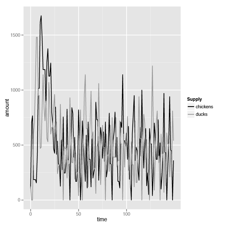
No surprises here. We can see that the supply of chickens and ducks alternates in highs and lows, confirming our earlier analysis. Next, we look at the comparison between the price of chickens and ducks. Just as with supply, we can guess that the prices will also alternate between chickens and ducks. This is because when the price of chickens goes up, more consumers will start buying ducks instead of chickens in the next turn. This will cause the duck supply to run low and the producers to increase their prices to maximize profit. In that same turn, though, because consumers are now buying ducks, the producers have no choice but to decrease the price of chickens.
Let’s look at the R script in Example 4-17.
Example 4-17. Comparing the prices of chickens and ducks
library(ggplot2)
data <- read.table("price_data.csv", header=F, sep=",")

ggplot(data = data) + scale_color_grey(name="Average price") +
  geom_line(aes(x  = V1, y = V2, color = "chickens")) +
  geom_line(aes(x  = V1, y = V3, color = "ducks")) +
  scale_y_continuous("price") +
  scale_x_continuous("time")
Again, this is very familiar territory, so we’ll just jump right ahead to the chart in Figure 4-4.
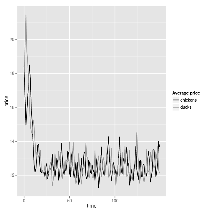
Again, we see the pattern of fluctuating prices for chickens and ducks. All pretty boring stuff by now. But wait—notice that the starting price of both chickens and ducks is quite high, but not long into the simulation, the prices competed with each other and dropped drastically until they both hit their costs, which is $12. This looks a lot like Figure 4-2. That’s still not very interesting, though; in fact, this seems very much like Example 4-9 in our first simulation where the price dropped to around cost.
You’re missing a very important point if you think that the results are boring. The fact that prices tend to drop to near cost shows that producers cannot set their prices arbitrarily. Very often, producers and merchants are accused of profiteering and arbitrarily setting up high prices in order to get as much profit as possible. While producers’ main motivation is primarily profit, in a free market economy it is usually difficult for them to set arbitrary prices that are overly high.
Of course, there are circumstances that do cause this—for example, if all the producers collude (a cartel), if a single producer has a monopoly, or if the market is a large geographically isolated location—which really only means that it’s not a free market economy. Given that the only difference between the two goods is the price, there is no choice but for the producers to drop their prices to stay competitive.
Having said that, remember that in our simulation the cost of producing chickens and ducks is the same. What if we increase the cost of producing ducks, meaning the difference is now not only the price?
COST[:ducks] = 24
COST[:chickens] = 12
Let’s see how doubling the cost of producing ducks affects the prices (Figure 4-5).
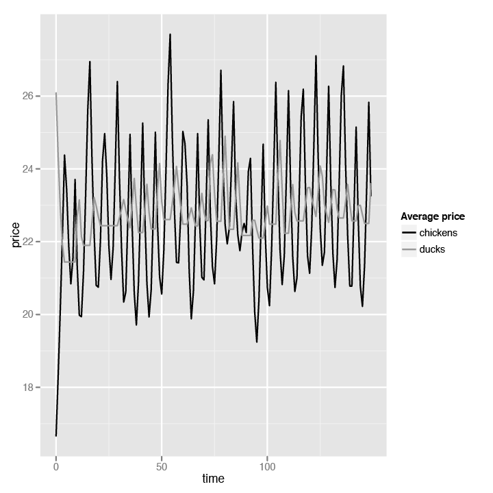
The basic patterns remain the same: the prices of chickens and ducks still alternate in highs and lows. However, notice that the stable price is now between $22 and $26—that is, centering the cost of ducks. This means that while ducks are being sold with marginal profit, chickens are sold with high profits! In that case, why don’t the farmers all sell chickens only? That doesn’t work, of course, since if everyone produces and sells chickens only, the stable price will be back at the level of our first simulation, which hovers around the cost of producing the chickens.
Price controls are not a new phenomenon. The idea that there is a “fair” price for certain goods, which can be determined by governments or rulers, has been around since early recorded history. As early as 2800 B.C., the ancient Egyptians strived to maintain grain prices. In Babylon, the famous Code of Hammurabi, the first ever written law code, imposed a rigid system of controls over wages and prices. In ancient China, the Rites of Zhou, a description of the organization of the government during the Western Zhou period (1046–256 B.C) laid down detailed regulations of commercial life and prices. In ancient Greece, an army of grain inspectors called Sitophylakes was appointed to set the price of grain to what the government thought just.
None of these structures was eventually successful, of course. In modern times, such price controls are often the promises made by politicians during their election campaigns, and just as often implemented to the short-lived joy of their electorate. A proven way to win the hearts of voters is to promise lower prices for goods. However, as we have seen earlier, changes in prices cannot be isolated and necessarily affect supply of the goods.
Let’s look at how price controls in our simulation affect our tiny market economy. We will be modifying our last simulation only slightly. First, we will add in the price control parameters:
PRICE_CONTROL = Hash.new
PRICE_CONTROL[:ducks] = 28
PRICE_CONTROL[:chickens] = 16
Notice that price control doesn’t really mean forcing the producers to produce below their cost. If that’s the case, even the dumbest politician will realize that no producer will produce and the whole economy will fail. In our example, the price control gives a bit of leeway for the producers to profit; for both the chickens and the ducks, the maximum profit that the producer will be able to get is $4. For most people, that would seem reasonable.
Now let’s modify a line in the Producer
class change_pricing method, as shown in Example 4-18.
Example 4-18. Adding the price control logic
def change_pricing
  @price.each do |type, price|
    if @supply[type] > 0
      @price[type] *= PRICE_DECREMENT unless @price[type] < COST[type]
    else
      @price[type] *= PRICE_INCREMENT unless @price[type] > PRICE_CONTROL[type]
    end
  end
end
In this code, we’re disallowing price increments if the price is above the price control level. That’s the only change there is. Now let’s run the code and see what happens.
After running the code, we’ll run the same analysis as in our previous simulation on price_data.csv and supply_data.csv. We don’t need to change the script, so let’s look at the chart for the price data (Figure 4-6).
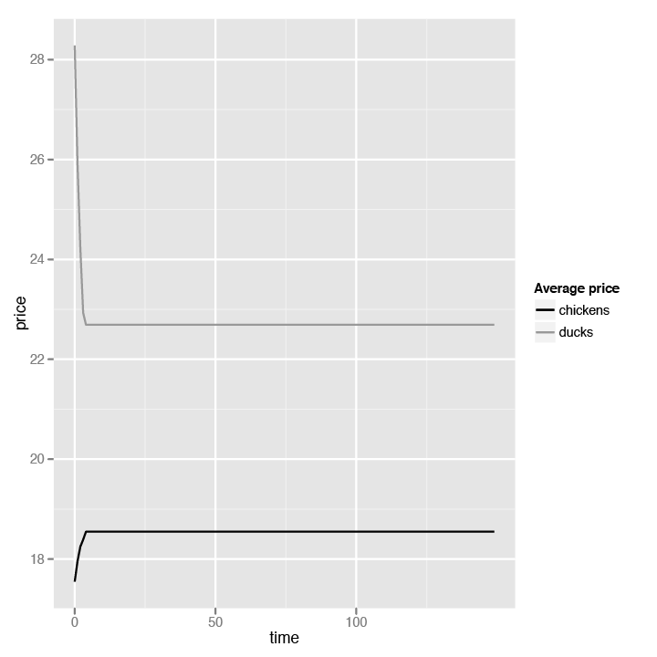
Drastic change! As you can see, the price of chickens stabilizes and doesn’t go beyond $20, and the price of ducks stabilizes and doesn’t go beyond $23. This is well and good, since that’s the intention of the price control. Now let’s look at the chart for the supply data (Figure 4-7).
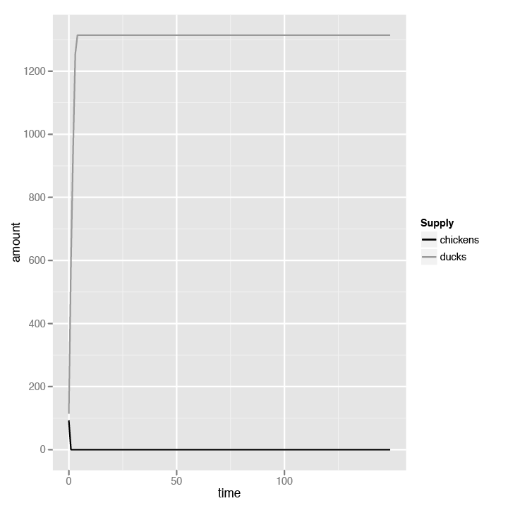
The devastation is obvious. After a turn or so, no farmers produce any chickens. Ducks can sell for more, so all farmers produce ducks. However, no consumer wants to buy ducks because chickens are cheaper, so the supply of ducks grows until it hits a ceiling, at which point both supplies stagnate until the end of the simulation. Our tiny chickens and ducks economy is broken.
Of course, our simulations are idealized, and as mentioned at the beginning of this chapter, simply models. However, they do give an indication of how price controls are fundamentally flawed. There are ways to get around the problems of our simulation (and in real life, no one is going to continually produce ducks if no one wants them, and neither will anyone give up eating because they can’t get the cheapest food), but they involve increasingly complex solutions that necessarily take from one side of the equation to give to the other side. While they might work under certain specialized circumstances, in a larger context and in the longer term, price controls almost never work.
This chapter provided only a brief glimpse into the world of economics modeling using software. We started with the most basic of economic theories and simulated a free market economy comprising a group of producers producing a single type of goods for a group of consumers.
The producers produce goods based on how well they sell. If the producers’ supply runs out, they will start producing. The producers also change their pricing based on how well their goods sell. If their goods are sold out, they will try to maximize their profits by increasing the price of their goods. If there are unsold goods, the producers will try to sell them off more aggressively by reducing their price. Of course, the producers will not reduce the price below the cost of producing the goods. The consumers consume based on their own demand, which fluctuates over time. They will consume from the producers with the cheapest goods until their demands are met.
We analyzed this simple simulation, and discovered as expected, that the supply for goods goes up when the demand goes down, and vice versa. We also showed that the price of goods stabilizes near the cost of producing the goods over time.
Our second simulation took our first and modified it for an economy of two types of goods—chickens and ducks. The basic rules set down in our first simulation were applied, and we analyzed the results. As it turned out, when the supply of chickens increased, the supply of ducks went down, and vice versa, as expected. Also, the price of goods stabilizes again over time.
However, we made the interesting discovery that if the cost of producing one type of goods is different from the other (in our case, the cost of producing ducks is higher than the cost of producing chickens), the prices will stabilize near the higher cost.
Finally, we ended this brief investigation and simulation by analyzing how price control affects our tiny economy. We learned that controlling and fixing the prices for ducks and chickens, while allowing some profit for the producers, is disastrous for the economy. One type of goods simply vanishes from the market because no producer wants to produce it anymore, while the other type goes unsold even though the prices are more reasonable than when a free market economy existed.
Economics modeling is a huge field, and what we’ve gone through in this chapter is less than even a scratch on the surface. I invite you to apply the tools and techniques you’ve learned here to dive deeper into this fascinating subject.
[9] This question originated in economist Charles Wheelan’s 2002 book Naked Economics (W. W. Norton & Company).
Get Exploring Everyday Things with R and Ruby now with the O’Reilly learning platform.
O’Reilly members experience books, live events, courses curated by job role, and more from O’Reilly and nearly 200 top publishers.

