Excel Hacks

Chapter 4. Hacking PivotTables

Hacks #46-49

PivotTables are one of Excel’s most powerful attractions, though many people don’t know what they do. PivotTables display and extract a variety of information from a table of data that resides within either Microsoft Excel or another compatible database type. PivotTables are frequently used to extract statistical information from raw data. You can drag around the different fields within a PivotTable to view its data from different perspectives.

Tip

The raw data for a PivotTable must be laid out in a classic table format. Row 1 of the table must be headings, with related data directly underneath. The data should not contain blank columns or blank rows. Even if you aren’t planning to use PivotTables, keeping your raw data in this format makes it possible for other people to analyze your data with PivotTables.

If you have not yet delved into the world of PivotTables, you should consider doing so. As a starting point, visit http://www.ozgrid.com/Excel/default.htm and work your way through Microsoft’s free online tutorial for Excel PivotTables. To learn even more about the benefits of PivotTables as well as how you can create hacks that make PivotTables even more flexible and powerful, read on.

PivotTables: A Hack in Themselves

PivotTables are one of the wildest but most powerful features of Excel, an ingenious hack themselves that may take some experimentation to figure out.

We use PivotTables a lot when we develop spreadsheets for our clients. Once a client sees a PivotTable, they nearly always ask whether they can create one themselves. Although anyone can create a PivotTable, unfortunately many people tend to shy away from them, as they see them as too complex. Indeed, when you first use a PivotTable, the process can seem a bit daunting. Some persistence is definitely necessary.

You’ll find that persistence will pay off once you experience the best feature of PivotTables: their ability to be manipulated using trial and error and immediately show the result of this manipulation. If the result is not what you expect, you can use Excel’s Undo feature and have another go! Whatever you do, you are not changing the structure of your original table in any way, so you can do no harm.

Why Are They Called PivotTables?

PivotTables allow you to pivot data using drag-and-drop techniques and receive results immediately. PivotTables are interactive; once the table is complete, you very easily can see how your information will be affected when you move (or pivot) your data. This will become patently clear once you give PivotTables a try.

Even for experienced PivotTable developers, an element of trial and error is always involved in producing desired results. You will find yourself pivoting your table a lot!

What Are PivotTables Good For?

PivotTables can produce summary information from a table of information. Imagine you have a table of data that contains names, addresses, ages, occupations, phone numbers, and Zip Codes. With a PivotTable, you very easily and quickly can find out:

• How many people have the same name

• How many people share the same Zip Code

• How many people have the same occupation

You also can receive such information as:

• A list of people with the same occupation

• A list of addresses with the same Zip Code

If your data needs slicing, dicing, and reporting, PivotTables will be a critical part of your toolkit.

Why Use PivotTables When Spreadsheets Already Offer So Much Analysis Capability?

Perhaps the biggest advantage to using PivotTables is the fact that you can generate and extract meaningful information from a large table of data within a matter of minutes and without using up a lot of computer memory. In many cases, you could get the same results from a table of data by using Excel’s built-in functions, but that would take more time and use far more memory.

Another advantage to using PivotTables is that if you want some new information, you can simply drag-and-drop (pivot). In addition, you can opt to have your information update each time you open the workbook or click Refresh.

PivotCharts Extend PivotTables

Microsoft introduced PivotCharts in Excel 2000. The table you create via the PivotTable Wizard produces a PivotChart (or, more accurately, a PivotTable and PivotChart Report). When you create a PivotTable, you also can create a PivotChart at the same time, with no extra effort. PivotCharts enable you to create interactive charts that previously were impossible without using either VBA or Excel Controls.

The PivotTable Wizard is discussed in more detail later in this chapter.

Tip

PivotCharts are not available in Excel for the Macintosh.

Creating Tables and Lists for Use in PivotTables

When you create a PivotTable, you must organize the dataset you’re using in a table and/or a list. As the PivotTable will base all its data on this table or list, it is vital that you set up your tables and lists in a uniform way.

In this context, a table is no more than a list that has a title, has more than one column of data, and has a different heading for each column. A list often is referred to in the context of a table as well. The best practices that apply to setting up a list will help you greatly when you need to apply a PivotTable to your data.

When you extract data via the use of lookup or database functions, you can be a little less stringent in how you set up the table or list. This is because you can always compensate with the aid of a function and probably still get your result. Nonetheless, it’s still easiest to set up the list or table as neatly as possible. Excel’s built-in features assume a lot about the layout and setup up of your data. Although they offer a degree of flexibility, more often than not you will find it easier to adhere to the following guidelines when setting up your table or list:

• Headings are required, as a PivotTable uses them for field names. Headings should always appear in the row directly above the data. Also, never leave a blank row between the data and the headings. Furthermore, make the headings distinct in some way; for instance, boldface them.

• Leave at least three blank rows above the headings. You can use these for formulas, critical data, etc. You can hide the rows if you want.

• If you have more than one list or table on the same worksheet, leave at least one blank column between each list or table. This will help Excel recognize them as separate entities. However, if the lists and tables are related to each other, combine them into one large table.

• Avoid blank cells within your data. Instead of leaving blank cells for the same data in a column, repeat the data as many times as needed.

• Sort your list or data, preferably by the leftmost column. This will make the data easier to read and interpret.

If you follow these guidelines as closely as possible, using PivotTables will be a relatively easy task.

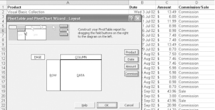
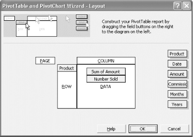
Figure 4-1 shows a well-laid out table of data, and a PivotTable in progress. Note that many of the same dates are repeated in the Date column. In front of this data is the Layout step for the data showing the optional Page, Row, and Column fields, as well as the mandatory Data field.

Figure 4-1. PivotTable generated from a well-laid out table of data

The PivotTable and PivotChart Wizard

As noted earlier, to help users create PivotTables, Excel offers a PivotTable and PivotChart Wizard. This Wizard guides you through the creation of a PivotTable using a four-step process, in which you tell Excel the following:

• How the data is set up and whether to create an associated PivotChart (if PivotCharts are available in that version of Excel)

• Where the data is stored—e.g., a range in the same workbook, a database, another workbook, etc.

• Which column of data is going into which field: the optional Page, Row, and Column fields, as well as the mandatory Data field

• Where to put your PivotTable (i.e., in a new worksheet or in an existing one)

You also can take many side steps along the way to manipulate the PivotTable, but most users find it easier to do this after telling Excel where to put it.

Tip

Excel 2000 and later versions have a major advantage over Excel 97: they enable you to choose how to set up your data after the Wizard is finished.

Now that you know more about PivotTables and what they do, it’s time to explore some handy hacks that can make this feature even more powerful.

Share PivotTables but Not Their Data

Create a snapshot of your PivotTable that no longer needs the underlying data structures.

You might need to send PivotTables for others to view, but for whatever reason you cannot send the underlying data associated with them. Perhaps you want others to see only certain data for confidentiality reasons, for instance. If this is the case, you can create a static copy of the PivotTable and enable the recipient to see only what he needs to see. Best of all, the file size of the static copy will be only a small percentage of the original file size.

Assuming you have a PivotTable in a workbook, all you need to do is select the entire PivotTable, copy it, and on a clean sheet select Edit → Paste Special... → Values. Now you can move this worksheet to another workbook or perhaps use it as is.

The one drawback to this method is that Excel does not paste the PivotTable’s formats along with the values. This can make the static copy harder to read and perhaps less impressive. If you want to include the formatting as well, you can take a static picture (as opposed to a static copy) of your PivotTable and paste this onto a clean worksheet. This will give you a full-color, formatted snapshot of the original PivotTable to which you can apply any type of formatting you want, without having to worry about the formatting being lost when you refresh the original PivotTable. This is because the full-color, formatted snapshot is not linked in any way to the original PivotTable.

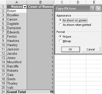
To create a static picture, format the PivotTable the way you want it and then select any cell within it. From the PivotTable toolbar, select PivotTable → Select → Entire Table. With the entire PivotTable selected, hold down the Shift key and select Edit → Copy → Picture. From the Copy Picture dialog box that pops up, make the selections shown in Figure 4-2, then click OK.

Figure 4-2. Copy Picture dialog in action

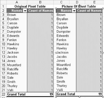
Finally, click anywhere outside the PivotTable and select Edit → Paste. You will end up with a fully colored and formatted snapshot of your PivotTable, as shown in Figure 4-3, complete with formatting. This can be very handy, especially if you have to email your PivotTable to other people for viewing. They will have the information they need, including all relevant formatting, but the file size will be small and they won’t be able to manipulate your data. Also, they will be able to see only what you want them to see.

Figure 4-3. Original PivotTable contrasted with a picture of the PivotTable

You also can use this picture-taking method on a range of cells. You can follow the preceding steps, or you can use the little-noticed Camera tool on your toolbar.

To use this latter method, select View → Toolbars → Customize.... From the Customize dialog, click the Commands tab, from the Categories box, select Tools, and from the Commands box on the righthand side scroll down until you see Camera. Left-click and drag-and-drop this icon onto your toolbar where you want it to be displayed. Select a range of cells, click the Camera icon, and then click anywhere on the spreadsheet, and you will have a linked picture of the range you just took a picture of. Whatever data or formatting you applied to the original range will automatically be reflected in the picture of the range.

Automate PivotTable Creation

The steps you need to follow to create a PivotTable require some effort, and that effort often is redundant. With a small bit of VBA, you can create simple PivotTables automatically.

PivotTables are a very clever and potent feature to use on data that is stored in either a list or a table. Unfortunately, the mere thought of creating a PivotTable is enough to prevent some people from even experimenting with them. Although some PivotTable setups can get very complicated, you can create most PivotTables easily and quickly. Two of the most commonly asked questions in Excel concern how to get a count of all items in a list, and how to create a list of unique items from a list that contains many duplicates. In this section, we’ll show you how to create a PivotTable quickly and easily that accomplishes these tasks.

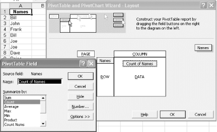
Assume you have a long list of names in column A, with cell A1 as your heading, and you want to know how many items are on the list, as well as generate a list of unique items. Select cell A1 (your heading) and then select Data → PivotTable and PivotChart Report (or Data → PivotTable Report on Macs) to start the PivotTable Wizard.

Make sure that either Microsoft Excel List or Database is selected, or that you have selected a single cell within your data. This will allow Excel to automatically detect the underlying data it is to use next. If you’re using a Windows PC, select PivotTable under “What kind of report do you want to create?” (This question isn’t asked on Macintoshes.) Click the Next button. The PivotTable Wizard should automatically have picked up the correct range for your data in column A and will highlight it in your sheet. If it is highlighted, click the Next button. Otherwise, use your mouse to select the range. Click the Layout button and drag to the Data area what will be your only field—you should see your title as it appears in cell A1 floating about. Drag the field again, this time into the Row area. Your screen should look something like Figure 4-4. Click OK.

Tip

At this stage, if you want you can double-click the Field button in the Data area (this is labeled Count of Names in Figure 4-3) and change the Summarize by: option to a function of your choice—e.g., Sum, Average, etc. Excel will by default use the COUNT function if it’s working with text and use the SUM function if it’s working with numbers.

Figure 4-4. PivotTable Field and PivotTable Layout dialogs

Finally, select New Worksheet as the destination of your PivotTable Report and click the Finish button. You should see your PivotTable on a new worksheet containing the unique items from your list along with a count of how many times each item (name) appears in your list.

What if you want to have a macro perform all those steps for you, creating a PivotTable from any column you feed it? If you simply record a macro, you’ll find it often works only if your data has the same heading. To avoid this, you can create a simple macro stored in your workbook or in your personal macro workbook (described in Chapter 7) that you can use to create a PivotTable on any list of items. This requires that you write some generic VBA code and enter it into a standard module in your personal macro workbook or in any other workbook.

To start, select Tools → Macro → Visual Basic Editor (Alt/Option-F11) and then select Insert → Module. Enter the following code:

Sub GetCount( )
Dim Pt As PivotTable
Dim strField As String

    strField = Selection.Cells(1,1).Text
    Range(Selection, Selection.End(xlDown)).Name = "Items"

    ActiveWorkbook.PivotCaches.Add(SourceType:=xlDatabase, _
    SourceData:="=Items").CreatePivotTable TableDestination:="", _
    TableName:="ItemList"
    
    Set Pt = ActiveSheet.PivotTables("ItemList")
     ActiveSheet.PivotTableWizard TableDestination:=Cells(3, 1)
     Pt.AddFields RowFields:=strField
     Pt.PivotFields(strField).Orientation = xlDataField

End Sub

To return to Excel, close the Script window, or press Alt/

-Q, and save your workbook.

Before running this code, select the heading of your list and ensure that your list contains no blank cells.

Tip

Sorting your list will remove blank cells quickly.

The code will automatically create a named range of your list, called Items. It will then create the PivotTable based on this named range on a new worksheet.

The next time you have a long list of data, you can simply select its heading and run this macro. All the PivotTable setup work will be done in the blink of an eye.

Move PivotTable Grand Totals

One of the most annoying things about PivotTables is that the Grand Total that summarizes your data always ends up at the bottom of the table, meaning you have to scroll down just to see the figures. Move your Grand Total up to the top where it’s easier to find.

Although PivotTables are a great way to summarize data and extract meaningful information, there is no built-in option to have the Grand Total float to the top for a quick bird’s-eye view.

Before we describe a very generic method to move the Grand Total to the top, we’ll explain how you can accomplish this with the GETPIVOTDATA function, which is designed specifically to extract data from a PivotTable.

You can use the function like this:

=GETPIVOTDATA("Sum of Amount",$B$5)

or like this:

=GETPIVOTDATA("Amount",$B$5)

Either function will extract the data and will track the Grand Total as it moves up, down, left, or right. We used the cell address $B$5, but as long as you use any cell within the PivotTable, you always will pick up the total.

The first function uses the Sum of Amount field, while the second one uses the Amount field. If your PivotTable has the Amount field in the Data area, you need to name the field Amount. If, however, the Amount field is being used two or more times in the Data area, you must specify the name you gave it, or the name you accepted by default (see Figure 4-5).

Figure 4-5. The Amount field used twice and named Sum of Amount in one case and Number Sold in the other

You can double-click these fields to change them. This issue can become confusing if you are not up to speed with PivotTables. Luckily in Excel 2002 and later, the process is much easier, as you can have a cell fill in the arguments and give the correct syntax by using the mouse pointer. In any cell, type = (an equals sign) and then use your mouse pointer to click in the cell currently housing the Grand Total. Excel will automatically fill in the arguments for you.

Warning

Unfortunately, if you use the Function Wizard, or first type =GETPIVOTDATA( ) and then click in the cell currently housing the Grand Total, Excel makes a mess by trying to nest another GETPIVOTDATA function within that cell.

Probably the easiest, if least sophisticated, way to extract the Grand Total is to use the following function:

=MAX(PivGTCol)

where the column currently housing the Grand Total is named PivGTCol.

You also can use the LARGE and SMALL functions to extract from a PivotTable a host of figures according to their size. The following formula, for instance, extracts the second largest figure from a PivotTable:

=LARGE(PivGTCol,2)

You can add some extra rows immediately above the start of the PivotTable and place these formulas there so that you can see this type of information instantly, without having to scroll to the bottom of your PivotTable.

Efficiently Pivot Another Workbook’s Data

Use data residing in another workbook as the source for your PivotTable.

When creating a PivotTable in Excel, you have lots of options for your data source. By far the easiest and most powerful approach is to use data that resides within the same workbook. Unfortunately, for whatever reason, this is not always possible or feasible. Perhaps the data that resides in another workbook is entered daily, for instance, and the users entering the data should not see the PivotTable.

Using a dynamic named range will greatly decrease the refresh time needed for your PivotTable to update. As you cannot reference a dynamic named range from another workbook, this also means you prevented the PivotTable from referencing perhaps thousands of blank rows and causing the file size to increase substantially. This way, you can pull in data from another workbook, and then base your PivotTable on the data in the same workbook rather than referencing it externally.

In the workbook that will contain your PivotTable, insert a new worksheet and call it Data. Open the workbook containing the data to be referenced, and ensure that the worksheet containing the data is the active sheet. In any spare cell on this worksheet, enter this formula:

=IF(A1="","",A1)

where A1 is the very first heading of your data table.

Select cell A1. Then cut it, activate your original workbook, and paste cell A1 in cell A1 on the Data sheet. This will give you the reference to the other workbook. Copy this cell across as many columns as there are headings in your data source. Then select Insert → Name → Define, and in the Names in Workbook: field, type PivotData. In the Refers to: box, type the following:

=OFFSET($A$1,0,0,COUNTA($A:$A),COUNTA($1:$1))

Click Add, then click OK. Next, to insert some code that will run each time the workbook is opened, right-click the Excel icon (located at the top left corner of the screen) and enter the following code:

Private Sub Workbook_Open( )
 With Worksheets("Data")
   .Range("2:1000").Clear
   .Range("1:1").AutoFill .Range("1:1000")
   .Range("2:1000") = .Range("2:1000").Value
 End With
End Sub

Tip

This shortcut isn’t available on a Mac. You’ll have to open the VBE by pressing Option-F11, or by selecting Tools → Macro → Visual Basic Editor. Then Ctrl-click This Workbook in the Projects window.

To return to Excel, close the script window or press Alt/

-Q.

The preceding code includes only 1,000 rows of data. This figure should always be greater than the number of rows you believe you will need. In other words, if your table in the other workbook contains 500 rows, add a few hundred more to accommodate any growth in the original table.

Warning

Avoid using an extremely high row number (like 10,000, unless you actually have that much data), as this will greatly impact how quickly the code runs and the data updates.

Save the workbook, close it, and then reopen it, making certain that you enabled macros. The code you added will fire automatically and will copy the formulas in row 1 on the Data sheet, then automatically convert all but row 1 into values only. This will leave you with a copy of your original data source, which will update each time you open the workbook.

Now you can hide this sheet if you want by selecting Format → Sheet → Hide or by using the method described in [Hack #5].

Now, to base a PivotTable on this dynamic named range, select anywhere within the PivotTable, then select the Wizard option from the PivotTable toolbar. Click the Back button until you reach Step 1 of the Wizard. Select the first option, Microsoft Excel List or Database, click Next, and in Step 2, type =PivotData (the name of the dynamic named range). Then click Finish.

You will not experience the lag that often occurs when a PivotTable is referencing an external data source because now the data itself is stored within the same workbook. As an added bonus, because you can use a dynamic named range, the PivotTable is dynamic without having to reference heaps of blank rows, and the file is kept to a manageable size.