I switch around a lot between fairly similar worksheets, and it would save me hours of hassle if I could move from one worksheet to another and keep my cursor in the same position in the new sheet as the one I just left.
Excel is designed to remember the last active cell on each worksheet, and to reactivate that cell when you open that sheet again. However, hereâs a macro you can use that will move you to the next worksheet in your workbook and place your cursor in the same active cell (it works in every version of Excel since Excel 97):
   Sub NextSheetSameCell()

   Dim rngCurrentCell As Range
   Dim shtMySheet As Worksheet
   Dim strCellAddress As String

   'strCellAddress = ActiveCell.Address

   'Comment out the line above to record the
   'selected range's address, or comment out the
   'line below to record the active cell's address.

   strCellAddress = _
    ActiveWindow.RangeSelection.Address

   Set shtMySheet = ActiveWindow.ActiveSheet

   If Worksheets.Count > shtMySheet.Index Then

    shtMySheet.Next.Activate
    Range(strCellAddress).Activate

    Else

    Worksheets(1).Activate
    Range(strCellAddress).Activate

   End If

   Set shtMySheet = Nothing

   End Sub
For good measure, I wrote the macro so that you can move to either the same active cell or the same range of selected cells as you move from worksheet to worksheet. In either case, the macro records the address of the selected cell or cells, activates the next worksheet in your workbook (or returns to the first worksheet if youâre currently on the last one), and applies the recorded selection to the new worksheet. To edit the macro so that you transfer only to the active cell (even if more than one cell is selected), put an apostrophe in front of the line that reads strCellAddress = ActiveCell.Address and remove the apostrophe from in front of the line that reads strCellAddress = ActiveWindow.RangeSelection.Address.
If you find the macro useful, you can attach it to a custom button on the toolbar. To find out how, see "Run a Macro by Clicking a Toolbar Button or Menu Item" in Chapter 8.
I have too much data in my worksheet to fit on a single screen. Can I shrink the contents of the window so that I can see everything at once?
You can control the relative size of the contents of the Excel window using the Zoom field in Excelâs standard toolbar. In the Zoom field on the toolbar (see Figure 1-15), click the down arrow and select a preset zoom value, or type a value directly into the field. The maximum zoom magnification is 400%; the minimum is 10%.
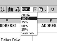
Figure 1-15. The Zoom field in the toolbar controls how large the body of your Excel worksheet appears in the Excel window. You can select prefab settings, or type in your own magnification.
Another way to shrink a worksheet thatâs too big to fit on one screen is to use a smaller font, and then resize the rows and columns to match:
Press Ctrl-A to select the entire worksheet, open the Font drop down on the toolbar, and select a smaller font.
While the entire sheet is still selected, choose Format â Column â AutoFit Selection.
While the entire sheet is still selected, choose Format â Row â AutoFit.
Iâm using a small range of cells in my worksheet, and Iâd like to see just those cells, displayed as large as possible. Iâve been trying to use the Zoom field, but I canât get it right. Am I out of luck?
Nope. Select the desired cells, and then follow these steps:
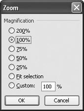
Choose View â Zoom to bring up the Zoom dialog box (as in Figure 1-16).
Click Fit Selection.
Click OK.
I just imported a database table into my worksheet, but I donât remember how many rows were in the table. I hate scrolling through my worksheets without knowing how far I have to go. Isnât there a way that I can just go directly to the last row of the list?
Press Ctrl-down arrow to go to the last cell used in the active column. You also can press Ctrl-up arrow to go to the first cell in the active column. Similarly, Ctrl-right arrow takes you to the last cell used in the active row, while Ctrl-left arrow selects the first cell used in the active row. Ctrl-End takes you to the bottom right corner of the worksheet; Ctrl-Home takes you to the very first cell (A1).
I have a data list with nine columns that run down for several hundred rows. When I scroll down, the headers that tell me which columns contain which data scroll off the top of the screen, so I canât figure out which column is which. My friend, who used to work on the other side of my cube wall, knew how to keep all the top row headings visible on her worksheets no matter how far down she scrolled. But she got a better offer from another company and left last week without teaching me the trick. How did she do that?
You can freeze one or more rows, columns, or both so that they remain visible when you scroll through a worksheet. To freeze one or more columns at the left edge of your worksheet, follow these steps:
Click the first cell in (or the column header of) the column to the right of the last column you want to freeze.
Choose Window â Freeze Panes.
To freeze one or more rows at the top edge of your worksheet, follow these steps:
Click the first cell in (or the row header of) the row below the last row you want to freeze.
Choose Window â Freeze Panes.
To freeze rows and columns along the top and left edges of your worksheet, follow these steps:
Click the cell below and to the right of the rows and columns you want to freeze (cell B3 in Figure 1-17).
Choose Window â Freeze Panes.
To unfreeze frozen rows and columns, choose Window â Unfreeze Panes.
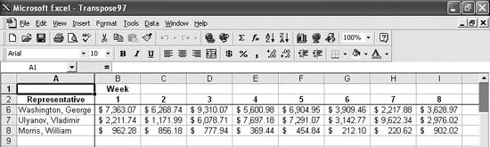
Figure 1-17. Itâs easier to read worksheet data when the row and column headings stay visible as you scroll.
Tip
You canât freeze columns and then freeze rows, or vice versa, using this technique. If you try, youâll see only the Unfreeze Panes item on the Window menu. To freeze columns and rows at the same time, you must click the cell below and to the right of the rows and columns you want to freeze.
You can create and manipulate these panes in freeform fashion using the mouse. Simply grab the small rectangular object just above the top arrow on the vertical scrollbar (the pointer changes to two lines with arrows on each side) and pull it down to just below the rows you want to freeze. Do the same with the small rectangular object just to the right of the right arrow on the horizontal scrollbar and drag it just to the left of the columns you want to freeze.
Iâm the executive editor at a major computer book publisher, so I build and maintain some huge Excel workbooks. Some of the worksheets span 10 or 12 printed pages, with the columns tracking the date we offered a book contract, the date the signed contract was returned, the date we took delivery of the authorâs first-born, that sort of thing. My problem: when I want to find a date in a certain column, or even within a cell range, Excel insists on searching the entire worksheet. Thereâs got to be a way to do pinpoint searching!
I sympathize with your plight, since I sufferâer, benefitâat the hands of editors every day. Fortunately, you can limit your search to an area of a worksheet by selecting that area before you choose Edit â Find. If you want to search a column, for example, click the corresponding column header. To search a swath of the worksheet, just paint it out with your mouse, press Ctrl-F (the keyboard shortcut), and search away. Excel will highlight (or rather, âreverseâ highlight) the found cell.
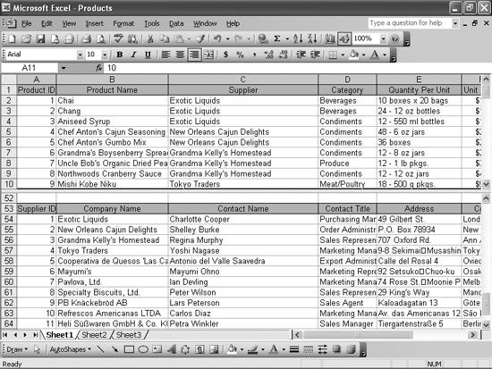
For some reason one of my co-workers put two different data sets on one worksheet. The first 50 rows hold data about our products, and rows 53â66 hold data about our suppliers. Moving either data set to another worksheet would mess up dozens of formulas in this and in other workbooks, but Iâd love to be able to scroll around in the product rows, keep whichever row I want from that area on the screen, and still display the suppliers rows. Is there some way to make that happen?
The trick is to divide your worksheet into two scrollable areas. Select the row below the last row you want in the top scrollable area, and choose Window â Split. The worksheet areas will have separate scrollbars, as shown in Figure 1-18, allowing you to view two entirely different areas of your worksheet at once.
You also can split the screen vertically using the same steps, except you select the column just to the right of the one you want in the left scrollable area.
To remove the split, choose Window â Remove Split.
While a workbook is split into panes, you can press F6 to move to the next pane in a clockwise direction, or press Shift-F6 to move to the next pane in a counter-clockwise direction.
Get Excel Annoyances now with the O’Reilly learning platform.
O’Reilly members experience books, live events, courses curated by job role, and more from O’Reilly and nearly 200 top publishers.

