Creating a basic worksheet is only the first step toward mastering Excel. If you plan to print your worksheet, email it to colleagues, or show it off to friends, you need to think about whether your worksheet is formatted in a viewer-friendly way. A careful use of color, shading, borders, and fonts can make the difference between a messy glob of data and a worksheet that’s easy to work with and understand.
But formatting isn’t just about deciding, say, where and how to make your text bold. Excel also lets you control the way numerical values are formatted. In fact, there are really two fundamental aspects of formatting in any worksheet:
Cell appearance. Cell appearance includes cosmetic details like color, typeface, alignment, and borders. When most people think of formatting, they think of cell appearance first.
Cell values. Cell value formatting controls the way Excel displays numbers, dates, and times. For numbers, this includes details like whether to use scientific notation, the number of decimal places displayed, and the use of currency symbols, percent signs, and commas. With dates, cell value formatting determines what parts of the date are shown in the cell, and in what order.
Cell value formatting is in many ways more significant than cell appearance, because it can change the meaning of your data. For example, even though 45%, $0.45, and 0.450 are all the same number, your spreadsheet readers will see a failing test score, a cheap price for chewing gum, and a world-class batting average, respectively.
Tip
Keep in mind that regardless of how you format your cell values, Excel maintains an unalterable value for every number entered. For more on how Excel internally stores numbers see the box on Sidebar 4.1.
In this chapter, you’ll learn about cell value formatting, and then unleash your inner artist with cell appearance formatting. Finally, you’ll learn the most helpful ways to use formatting to improve a worksheet’s readability and how to save time with nifty features like AutoFormat, styles, and conditional formatting.
Cell value formatting is one aspect of worksheet design you don’t want to ignore, because the values Excel stores can differ from the numbers that it displays in the worksheet, as shown in Figure 4-1. In many cases, it makes sense to have the numbers that appear in your worksheet differ from Excel’s underlying values, since a worksheet that’s displaying numbers to, say, 13 decimal places, can look pretty cluttered.
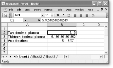
Figure 4-1. This worksheet shows how different formatting can affect the appearance of the same data. Each of the cells B2, B3, and B4 contains the exact same number: 5.18518518518519. Excel will always display in the Formula bar the exact number it’s storing, as you see here with cell B2. However, in the worksheet itself, each cell’s appearance differs depending on how you’ve formatted the cell.
To format a cell’s value, follow these steps:
Select the cells you want to format.
You can apply formatting to individual cells, or to a collection of cells. Usually, you’ll want to format an entire column at once, because all the values in a column typically contain the same type of data. Remember, to select a column, you simply need to click the column header (the gray box at the top with the column letter).
Note
Technically, a column contains two types of data: the values you’re storing within the actual cells and the column title in the topmost cell (where the text is). However, you don’t need to worry about unintentionally formatting the column title because number formats are only applied to numeric cells (cells that contain dates, times, or numbers). Excel doesn’t use the number format for the column title cell because it contains text.
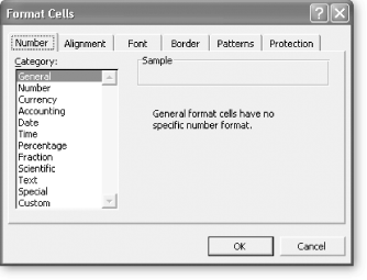
Select Format → Cells, or just right-click the selection, and choose Format Cells.
In either case, the Format Cells dialog box appears, as shown in Figure 4-2.
Figure 4-2. The Format Cells dialog box provides one-stop shopping for cell value and cell appearance formatting. The first tab, Number, lets you configure how numeric values are formatted. The Alignment, Font, Border, and Patterns tabs are all used to control the appearance of the cell. Finally, the Protection tab allows you to prevent changes and hide formulas. (You’ll learn about worksheet protection features in Chapter 13.)
Set the format options, and then click OK to apply them.
The options in the Number tab let you choose how Excel translates the cell value into a display value. (Number formatting choices are covered in the next section, Section 4.1.1.) Most of the other tabs on this dialog box are for cell appearance formatting, which is covered later in this chapter.
Note
Once you apply formatting to a cell, it retains that formatting even if you clear the cell’s contents (by selecting it and pressing Delete). In addition, formatting follows a cell copy, so if you copy the content from cell A1 to cell A2, the formatting comes with it. Formatting includes both cell value formatting and cell appearance.
The only way to remove the formatting is to highlight the cell and select Edit → Clear → Formats. This command removes the formatting, restoring the cell to its original, General number format (which you’ll learn more about next), but it doesn’t remove any of the cell’s content.
The Number tab in the Format Cells dialog box lets you control how Excel displays numeric data in a cell. Excel gives you a lengthy list of predefined formats (as shown in Figure 4-3), and it also lets you design your own formats. Remember, Excel uses number formats when the cell contains numeric information only. Otherwise, Excel simply ignores the number format (although the format is still there and will still be used if you change the cell content to a number, date, or time).

Figure 4-3. A good way to learn about the different number formats is to select a cell that already has a number in it and then choose a new number format from the Category list (select Format → Cell). When you do so, Excel uses the Format Cells dialog box to show how the number will be displayed if you apply that format. In this example, you can see that the cell value, 5.18518518518519, will appear as 5.19E+00, which is scientific notation with two decimal places.
When you create a new spreadsheet, every cell starts out with the same number format: General. This format comes with a couple of basic rules:
If a number has any decimal places, Excel displays them, provided they fit in the column. If there are more decimal places than Excel can display, it leaves out the ones that don’t fit. (It rounds up the last displayed digit, when appropriate). If you change a column width, Excel automatically adjusts the amount of digits it displays.
Excel removes leading and trailing zeros. Thus, 004.00 becomes 4. The only exception to this rule occurs with numbers between -1 and 1, which retain the 0 before the decimal point. For example, Excel displays the number .42 as 0.42.
As you saw in Chapter 2, the way you type in a number can change a cell’s formatting. For example, if you enter a number with a currency symbol, the number format of the cell changes automatically to Currency. Similarly, if you enter three numbers separated by dashes (-) or backward slashes (/), Excel assumes you’re entering a date, and adjusts the number format to Date.
However, rather than rely on this automatic process, it’s far better just to enter ordinary numbers and set the formatting explicitly for the whole column. This approach prevents you from having different formatting in different cells (which can confuse even the sharpest spreadsheet reader), and it makes sure you get exactly the formatting and precision you want. You can apply formatting to the column before or after you enter the numbers. And it doesn’t matter if a cell is currently empty; Excel still keeps track of the number format you’ve applied.
Different number formats provide different options. For example, if you choose Currency format, you can choose from dozens of currency symbols. If you use Number format, you can choose to add commas (to separate groups of three digits) or parentheses (to indicate negative numbers). Most number formats let you set the number of decimal places.
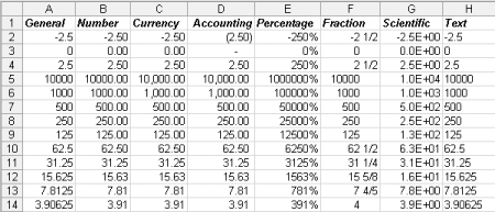
The following sections give a quick tour of the predefined number formats available in the Number tab in the Format Cells dialog box. Figure 4-4 gives you an overview of how different number formats affect similar numbers.
The General format is Excel’s standard number format; it applies no special formatting other than the basic rules described at the beginning of this chapter. General is the only number format (other than Text) that doesn’t limit your data to a fixed number of decimal places. That means if you want to display numbers that differ wildly in precision (like 0.5, 12.334, and 0.120986398), it makes sense to use General format. On the other hand, if your numbers have a similar degree of precision (for example, if you’re logging the number of miles you run each day), Number format makes more sense.
The Number format is like the General format but with three refinements. First, it uses a fixed number of decimal places (which you set). That means that the decimal point always lines up (assuming you’ve formatted an entire column). The Number format also allows you to use commas as a separator between groups of three digits, which is handy if you’re working with really long numbers. Finally, you can choose to have negative numbers displayed with the negative sign, in parentheses, or in red lettering.
The Currency format closely matches the Number format, with two differences. First, you can choose a currency symbol (like the dollar sign, pound symbol, Euro symbol, and so on) from an extensive list; Excel will display the currency symbol before the number. Second, the Currency format always includes commas. The Currency format also supports a fixed number of decimal places (chosen by you), and it allows you to customize how negative numbers are displayed.
The Accounting format is modeled on the Currency format. It also allows you to choose a currency symbol, uses commas, and has a fixed number of decimal places. The difference is that the Accounting format uses a slightly different alignment. The currency symbol is always shown at the far left of the cell (away from the number), and there is always an extra space that pads the right side of the cell. Also, the Accounting format always shows negative numbers in parentheses, which is an accounting standard. Finally, the number 0 is never shown when using the Accounting format. Instead, a dash (-) is displayed in its place.
The Percentage format displays fractional numbers as percentages. For example, if you enter 0.5, that translates to 50%. You can choose the number of decimal places to display.
There’s one trick to watch out for with the Percentage format. If you forget to start your number with a decimal, Excel quietly “corrects” your numbers. For example, if you type 4 into a cell that uses the Percentage format, Excel interprets this as 4%. As a result, it actually stores the value 0.04. A side-effect of this quirkiness is that if you want to enter percentages larger than 100%, you can’t enter them as decimals. For example, to enter 200%, you need to type in 200 (not 2.00).
The Fraction format displays your number as a fraction instead of a number with decimal places. The Fraction format doesn’t mean you have to enter the number as a fraction (although you can if you want by using the backward slash, like 3/4). Instead it means that Excel will convert any number you enter and display it as a fraction. Thus, to have 1/4 appear you can either enter .25 or 1/4.
The Fraction format is often used for stock market quotes, but it’s also handy for certain types of measurements (like weights and temperatures). When using the Fraction format, Excel does its best to calculate the closest fraction, which depends on a few factors including whether an exact match exists (entering .5 will always get you 1/2, for example) and what type of precision level you’ve picked when selecting the Fraction formatting.
You can choose to have fractions with three digits (for example, 100/200), two digits (10/20), or just one digit (1/2), using the top three choices in the Type list. For example, if you enter the number 0.51, Excel shows it as 1/2 in one-digit mode, and the more precise 51/100 in three-digit mode. In some cases, you might want all numbers to use the same denominator (the bottom number in the fraction) so that it’s easy to compare different numbers. In this case, you can choose to show all fractions as halves (with a denominator of 2), quarters (a denominator of 4), eighths (8), sixteenths (16), tenths (10), and hundredths (100). For example, the number 0.51 would be shown as 2/4 if you chose quarters.
Tip
Sometimes, entering a fraction in Excel can be awkward because Excel may attempt to convert it to a date. To prevent this confusion, always start by entering 0 and then a space. For example, instead of typing 2/3 enter 0 2/3 (which means zero and two-thirds). If you have a whole number and a fraction, like 1 2/3, you’ll also be able to duck the date confusion.
The Scientific format displays numbers using scientific notation, which is ideal when you need to handle numbers that range widely in size (like 0.0003 and 300) in the same column. Scientific notation displays the first non-zero digit of a number, followed by a fixed number of digits, and then indicates what power of 10 that number needs to be multiplied by to generate the original number. For example, 0.0003 becomes 3.00 10-4 (displayed in Excel as 3.00E-04). The number 300, on the other hand, becomes 3.00 102 (displayed in Excel as 3.00E02). Scientists—surprise, surprise—like the Scientific format for doing things like recording experimental data or creating mathematical models to predict when an incoming meteor will graze the Earth.
Few people use the Text format for numbers, but it’s certainly possible to do so. The Text format simply displays a number as though it were text, although you can still perform calculations with it. Excel shows the number exactly as it’s stored internally, positioning it against the left edge of the column. You can get the same effect by placing an apostrophe before the number (although that approach won’t allow you to use the number in calculations).
To format dates and times, in the Format Cells dialog box (Format → Cells), shown in Figure 4-5, choose Date or Time from the column on the left and then choose the format from the list on the right. Date and Time both provide a slew of options. You can use everything from compact styles like 3/13/05 to longer formats that include the day of the week, like Sunday, March 13, 2005. Time formats give you a similar range of options, including the ability to use a 12-hour or 24-hour clock, show seconds, show fractional seconds, and include the date information.
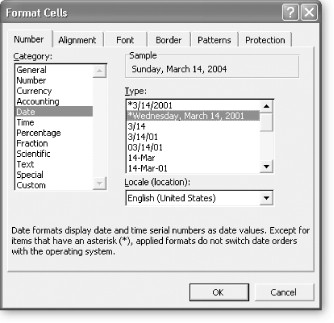
Figure 4-5. Excel gives you dozens of different ways to format dates and times. You can choose between formats that modify the date’s appearance depending on the regional settings of the computer viewing the Excel file or you can choose a fixed date format. When using a fixed date format, you don’t have to stick to the U.S. standard. Instead, choose the appropriate region from the Locale list box. Each locale provides its own set of customized date formats.
There are essentially two types of date and time formats:
Formats that take the regional settings of the computer you’re using into account. With these formats, dates display differently depending on the computer that’s running Excel. This is a good choice because it lets everyone see dates in just the way they want to, which means no time-consuming arguments about month-day-year or day-month-year ordering.
Formats that ignore the regional settings of individual computers. These formats define a fixed pattern for month, day, year, and time components, and display date-related information in exactly the same way on all computers. If you need to absolutely make sure a date is in a certain format, you should use this choice.
The first group (the formats that rely on a computer’s regional settings) is the smallest. It includes two date formats (a compact number-only format and a long, more descriptive format) and one time format. In the Type list, these formats are at the top and have an asterisk next to them.
The second group (the formats that are independent of a computer’s regional settings) is much more extensive. In order to choose one of these formats, you first select a region from the Locale list, and then you select the appropriate date or time format. Some examples of locales include “English (United States)” and “English (United Kingdom).”
If you enter a date without specifically formatting the cell, Excel usually uses the short region-specific date format. That means that the order of the month and year vary depending on the regional settings of the current computer. But if you incorporate the month name (for example, January 1, 2005), instead of the month number (for example, 1/1/2005), Excel uses a medium date format that includes a month abbreviation, like 1-Jan-2005.
Tip
You may remember from Chapter 2 that Excel stores a date internally as the cumulative number of days that have elapsed since a certain long-ago date that varies by operating system. You can take a peek at this internal number using the Format Cells dialog box. First, enter your date. Then, format the cell using one of the number formats (like General or Number). The underlying date number will appear in your worksheet where the date used to be.
There are some types of numeric information that you wouldn’t ever want to perform mathematical operations with. For example, it’s hard to image a situation where you’d want to add or multiply phone numbers or social security numbers.
When entering these types of numbers, therefore, you might choose to format them as plain old text. For example, you could enter the text (555) 123-4567 to represent a phone number. Because of the parentheses and the dash (-), Excel won’t interpret this information as a number. Alternatively, you could just precede your value with an apostrophe (') to explicitly tell Excel that it should be treated as text (you might do this if you don’t use parentheses or dashes in a phone number).
But whichever solution you choose, you’re potentially creating more work for yourself because you have to enter the parentheses and the dash for each phone number you enter (or the apostrophe). You also increase the likelihood of creating inconsistently formatted numbers, especially if you’re entering a long list of them. For example, some phone numbers might end up entered in slightly similar but somewhat different formats, like 555-123-4567 and (555)1234567.
To avoid these problems, apply Excel’s Special number format, as shown in Figure 4-6, which converts numbers into common patterns. And lucky you: one of the Type options in the Special number format is Phone Number (other formats are for Zip Codes and social security numbers).
The Special format is a good idea, but it’s limited. Out of the box, Excel only provides a small set of special types that you can use. However, there’s no reason you can’t handle similar problems by creating your own custom formats, as you’ll see in the next section.
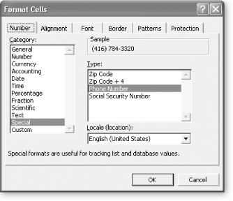
Figure 4-6. Special number formats are ideal for formatting sequences of digits into a common pattern. For example, if you choose Phone Number in the Type list, Excel converts the sequence of digits 5551234567 into the proper phone number style—(555) 123-4567—with no extra work required on your part.
As versatile as Excel is, it can’t read your mind. There are some situations when you want to format numbers in a specialized way that Excel just doesn’t expect. For example, you might want to use the ISO (International Organization for Standardization) format for dates, which is used in a wide range of scientific and engineering documents. This format is year-month-day (as in 2006-12-25). Although it’s fairly straightforward, Excel doesn’t provide this format as a standard option.
Or maybe you want to type in short versions of longer numbers. For example, say your company, International Pet Adventures, uses an employee number to identify each worker, in the format 0521-1033. It may be that 0521- is a departmental identification code for the Travel department. To save effort, you want to be able to enter 1033 and have Excel automatically insert the leading 0521- in your worksheets.
The solution lies in creating your own custom formats. Custom formats are a powerful tool for taking control of how Excel formats your numbers. Unfortunately, they aren’t exactly easy to master.
The basic concept behind custom formats is that you define the format using a string of special characters and placeholders. This format string tells Excel how to format the number or date, including details like how many decimal places it should include, and how it should treat negative numbers. You can also add fixed characters that never change, like the employee number format just described.
Here’s the easiest way to apply a custom format:
Select the cells you want to format.
This can include any combination of cells, columns, rows, and so on. To make life easier, make sure the first cell you select contains a value you want to format. That way, you’ll be able to use the Format Cells dialog box to preview the effect of your custom format.
Select Format → Cells, or just right-click the selection, and choose Format Cells.
The Format Cells dialog box appears, as shown earlier in Figure 4-2.
Choose a format that’s similar to the format you want to use.
For example, if you want to apply a custom date format, begin by selecting the Date number format and choosing the appropriate style. If you want to apply a custom currency format, begin by selecting the Currency number format and specifying the appropriate options (like the number of decimal places).
To create the International Pet Adventures employee code, it makes sense to first select the Number format, and then choose 0 decimal places (since the number format you’re looking to model—0521-1033—doesn’t use any decimal places).
At the bottom of the Category list, click Custom.
Now you’ll see a list of different custom number strings. At the top of this list is a highlighted format string that’s based on the format you chose in step 3. Now, you just need to modify this string to customize the format. (Make sure you don’t accidentally select another format before you click Custom, or you won’t end up with the right format string.)
If you’re creating the International Pet Adventures employee code, you’ll see a 0. This means you can use any number without a decimal place. However, what you really want in this situation is to create an employee number that always starts with 0521- and then has four more digits. You’ll specify your new format in the next step.
Enter your custom string.
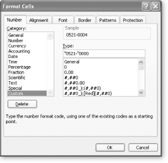
Type your custom string into the box below the Type label; Figure 4-7 shows the custom format string in the Format Cells dialog box. The correct format string for the International Pet Adventures example is as follows:
"0521-"0000
This string specifies that all cells that are formatted using this Custom format will begin with the digits 0521- and will then be followed by whatever four numbers are entered into the cell (if no numbers are entered, four zeroes will follow the 0521-). Page Section 4.1.4.2 explains all the ingredients you can use in your custom format.
Figure 4-7. Custom number strings allow you to do almost anything with a number format, but you’ll need to spell it out explicitly using the cryptic code Excel provides. In the example shown here, the format string is “0521-"0000. The “0521-” is a fixed string of characters that’s added to the beginning of every number. The four zeroes indicate that you need four digits. If you provide a one-, two-, or three-digit number, Excel will add the zeroes needed to make a four-digit number. For example, the number 4 will automatically be displayed as the employee code 0521-0004.
Click OK to commit your changes
If the results don’t meet with your approval, you can start over again. But this time, skip step 3, because you want to change the current format string rather than replace it with a new format string.
To use the Custom format you’ve created, select one or more cells, pick the Custom format (by right-clicking the cells and choosing Format Cells...), and then select your new Custom format.
Newly created Custom formats are listed in the Custom category, at the bottom of the Type list. If you wanted to use the new International Pet Adventures employee code, click OK after selecting your new format and then begin entering the four digits specific to each employee. For example, if you format a cell with the new Custom format, and you then type 6754 into the cell, you’ll see 0521-6754.
The tricky part about Custom formats is creating the right format string. To the untrained eye, the format string looks like a cryptic jumble of symbols—which it is. But these symbols, or formatting codes in Excel lingo, actually have very specific and clear meanings.
For example, the format string $#,##0.00 translates into the following series of instructions:
$ tells Excel to add a currency symbol before the number.
#,## tells Excel to use commas to separate thousands.
0.00 tells Excel to always include a single digit and two decimal places, no matter what the number is (0.00).
$#,##0.00 is the format string for the basic Currency format. Once you understand what the codes stand for and how they work together, you can create some really useful Custom format strings.
You have three types of codes at your disposal for creating format strings: those used to format dates and times; those used to format numbers; and those used to format ordinary text. The following three sections tackle each type of format code.
Date and time format strings are built out of pieces. Each piece represents a single part of the date, like the day, month, year, minute, hour, and so on. You can combine these pieces in whatever order you want, and you can insert your own custom text along with these values.
Note
Keep in mind that none of these formatting codes actually generate or insert the date in your worksheet for you. That is, simply formatting an empty cell with one of these custom strings isn’t going to cause the date to appear (although Excel can automatically insert dates; see Section 10.2 for more on that). Instead, these format strings take the dates that you enter and make sure that they all appear in a uniform style.
The basic ingredients for a date or time format string are shown in Table 4-1. These are placeholders that represent the different parts of the date. If you want to include fixed text along with the date, put it in quotation marks. For example, consider the following format string:
yyyy-mm-dd
Table 4-1. Date and Time Formatting Codes
|
Code |
Description |
Example Value Displayed on Worksheet[1] |
|---|---|---|
|
d |
The day of the month, from 1 to 31, with the numbers between 1 and 9 appearing without a leading 0. |
7 |
|
dd |
The day of the month, from 01 to 31 (leading 0 included from 1 to 9). |
07 |
|
ddd |
A three-letter abbreviation for the day of the week. |
Fri |
|
dddd |
The full name of the day of the week. |
Friday |
|
m |
The number value, from 1 to 12, of the month (no leading 0 used). |
1 |
|
mm |
The number value, from 01 to 12, of the month (leading 0 used for 01 to 09). |
01 |
|
mmm |
A three-letter abbreviation for the month. |
Jan |
|
mmmm |
The full name of the month. |
January |
|
yy |
A two-digit abbreviation of the year. |
05 |
|
yyyy |
The year with all four digits. |
2005 |
|
h |
The hour, from 0 to 23 (no leading 0 used). |
13 |
|
hh |
The hour, from 00 to 23 (leading 0 used from 00 to 09). |
13 |
|
:m |
The minute, from 0 to 59. |
5 |
|
:mm |
The minute, from 0 to 59 (leading 0 used for 00 to 09). |
05 |
|
:s |
The second, from 0 to 59 (no leading 0 used). If you want to add tenths or hundredths of a second, follow this with .0 or.00, respectively. For example, :s. |
5 |
|
:ss |
The second, from 0 to 59 (leading 0 used from 00 to 09). If you want to add tenths or hundredths of a second, follow this with .0 or .00, respectively. |
05 |
|
AM/PM |
Tells Excel to use a 12-hour clock, including the AM or PM tag. |
PM |
|
am/pm |
Tells Excel to use a 12-hour clock, with an am or pm tag. |
pm |
|
A/P |
Tells Excel to use a 12-hour clock, with an A or P tag. |
P |
|
a/p |
Tells Excel to use a 12-hour clock, with an a or p tag. |
P |
|
[ ] |
Tells Excel that a given time component (hour, minute, or second) shouldn’t “roll over.” For example, Excel’s standard approach is to have seconds become minutes once they hit the 60 mark, and minutes become hours at the 60 mark. Similarly, hours roll over into a new day when they hit 24. But if you don’t want this to happen—for example, when tracking total minutes on a CD play list—you could use the format string [h]:[mm]:ss. Thus, if your total play time were 59:59 (59 minutes and 59 seconds), and you added a 3 minute long song, the new total would be 62:59, rather than 1:02:59. | |
[1] Assumes the date January 7, 2005, 1:30:05 PM. | ||
Note
Regardless of how you type in the date, once you’ve formatted a cell using a Custom format string, that always overrides the format you use when you type in the date. In other words, it doesn’t matter if you type 1/15/06 or January 15, 2006 in the cell—Excel still displays it as 2006-01-15 if that’s what your custom format dictates.
If you apply this format string to a cell that contains a date, you’ll end up with the following in your worksheet (assuming you entered the date January 15, 2006): 2006-01-15.
Now if you format the same value with this format string:
"Day" yyyy-mm-dd
you’ll see this in your worksheet:
Day 2006-01-15
Whatever information you choose to display or hide, Excel always stores the same date internally.
Note
You’ll learn much more about date and time calculations in Chapter 10.
Custom number formats are more challenging than Custom date formats because Excel gives you lots of flexibility when it comes to customizing number formats. Table 4-2 shows the different codes you can use. The most important of these are the digit placeholders 0, ?, and #. You use these to tell Excel where it should slot in the various digits of the number that’s currently in the cell (or that you’re typing in).
Table 4-2. Number Formatting Codes
Note
Excel uses custom number formats to decide how to round off displayed numbers, and how to format them (by adding commas, currency symbols, and so on). But no matter what format string you use, you can’t coax Excel into shaving off digits that appear to the left of the decimal place—and for good reason—doing so would mangle your numbers beyond recognition.
Use 0 to indicate a number that must be wherever the 0 is placed—if it’s not, Excel automatically inserts a 0. For example, the format string 0.00 would display the number .3 as 0.30. And the format string 00.00 would format the same value as 00.30.
The question mark (?) works similarly, but it turns into spaces instead of zeroes, ensuring that multiple numbers wind up aligned in a column. For example, ??.?? displays the number 3 as " 3 " (without the quote marks).
The # symbol lets you indicate where a number can exist but doesn’t have to exist. For example, the format string 0.0# indicates that the first digit before the decimal place and the first digit after the decimal place must be present (that’s what the zeroes tell Excel). However, the second number after the decimal place is optional. With this format string, Excel rounds additional digits starting with the third decimal place. Thus, this format string will display the value .3 as 0.3, .34 as 0.34, and .356 as 0.36. You can also use the # symbol to indicate where commas should go, as in the format string #,##.00. This string will display the value 3639 as 3,639.00.
Note
Remember, Custom format strings control how values are displayed. They aren’t meant to control what values a person is allowed to enter in a cell. To set rules for allowed data, you need a different feature—data validation, which is described on Section 15.4.1.
Excel also lets you use codes that apply currency symbols, percent symbols, and colors. As with date values, you can insert fixed text—also known as literals— into a number formatting string using quotation marks. For example, you could add “USD” at the end of the format string to indicate that a number is denominated in U.S. dollars. Excel automatically recognizes some characters as literals, including currency symbols, parentheses, plus (+) and minus (-) symbols, backward slashes (/), and spaces, which means you don’t need to use quotation marks to have characters appear.
Finally, the last thing you should know about Custom number format strings is that if you’d like your worksheet to display different types of values (e.g., negative versus positive) differently, you can actually create a collection of four different format strings, each of which formats different types of numbers, depending on what values you type into the cell. Collectively, these four format strings tell Excel how to deal with positive values, negatives values, zero, and text values. The format strings must always appear in this order and be separated by semicolons. Here’s an example:
#,###; [red]#,###; "---"; @
Excel uses the first format string (#,###) if the cell contains a positive number. Excel uses the second format string ([red]#,###) to display negative numbers. This format is the same as for positive numbers, except it displays the text in red. The third format string (“—-”) applies to zero values. It inserts three dashes into the cell when the cell contains the number 0. (If the cell is empty, no format string is used, and the cell remains blank.) Finally, Excel uses the last format if you enter text into the cell. The @ symbol simply copies any text into the cell as it’s entered.
Tip
For a real trick, use the empty format string ; ; ; to puzzle friends and coworkers. This format string specifies that no matter what the content in the cell (positive number, negative number, zero, or text), Excel shouldn’t display it. The result is that you can add information to the cell (and see it in the Formula bar), but it won’t appear on the worksheet or in your printouts.
Text format strings are extremely simple. Usually, you use a text format string to repeatedly insert the same text in a large number of cells. For example, you might want to add the word NOTE before a collection of entries. To do this, your format string needs to define the literal text you want to use—in this case, the word “NOTE”—and place the text within quotation marks (including any spaces you wish to appear). Use the @ symbol to indicate which side of the string the cell contents should go. For example, if you set the format string:
"NOTE: "@
and then you type Transfer payment into the cell, Excel will display it as NOTE: Transfer payment.
Formatting cell values is important since it helps maintain consistency among your numbers. But to really make your spreadsheet readable, you’re probably going to want to enlist some of Excel’s tools for controlling things like alignment, color, and borders and shading.
To format the appearance of a cell, first select the single cell or group of cells that you want to work with, and then choose Format → Cells from the menu, or just right-click the selection and choose Format Cells. The Format Cells dialog box that appears is the place where you adjust your settings.
Note
Even a small amount of formatting can make a worksheet easier to interpret by drawing the viewer’s eye to important information. Of course, as with formatting a Word document or designing a Web page, a little goes a long way. Don’t feel the need to bury your worksheet in exotic colors and styles just because you can.
As you learned in the previous chapter, Excel automatically aligns cells according to the type of information you’ve entered. But what if this default alignment isn’t what you want? Fortunately, the Alignment tab in the Format Cells dialog box lets you easily change alignment as well as control some other interesting settings, like the ability to rotate text.
Excel lets you control the position of content between a cell’s left and right borders, offers the following choices, some of which are shown in Figure 4-8:
General. General is the standard type of alignment; it aligns cells to the right if they hold numbers or dates and to the left if they hold text. This is the type of alignment you learned about in Chapter 2.
Left (Indent). Left indicates that Excel should always line up content with the left edge of the cell. You can also choose an indent value to add some extra space between the content and the left border.
Center . Center indicates that Excel should always center content between the left and right edges of the cell.
Right (Indent). Right indicates that Excel should always line up content with the right edge of the cell. You can also choose an indent value to add some extra space between the content and the right border.
Fill. The Fill setting copies content multiple times across the width of the cell, which is almost never what you want.
Justify. This is the same as Left if the cell content fits on a single line. If you insert text that spans more than one line, Excel justifies every line except the last one, which means Excel adjusts the space between words to try and ensure that both the right and left edges line up.
Center Across Selection. This setting is a bit of an oddity. If you apply this option to a single cell, it has the same effect as Center. If you select more than one adjacent cell in a row (for example, cell A1, A2, A3), this option centers the value in the first cell so that it appears to be centered over the full width of all cells. However, this only happens as long as the other cells are blank. Because this setting can lead (confusingly) to cell values displaying over cells that they aren’t stored in, it’s usually not a good idea to use. A better approach to centering large text titles and headings is to use cell merging (as described on Sidebar 4.3).
Distributed (Indent). This is the same as Center if the cell contains a numeric value or a single word. If you add more than one word, Excel enlarges the spaces between words so that the text content fills the cell perfectly (from the left edge to the right edge).
Vertical alignment controls the position of content between a cell’s top and bottom border. Vertical alignment only becomes important if you enlarge a row’s height so that it becomes taller than the contents it contains. To change the height of a row, click on the bottom edge of the row header (the numbered cell on the left side of the worksheet), and drag it up or down. As you resize the row, the content stays fixed at the bottom. The vertical alignment setting lets you adjust the cell content’s positioning.
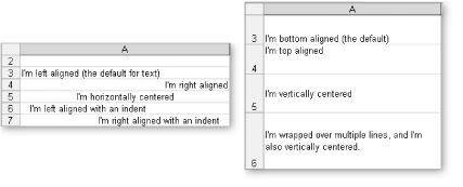
Figure 4-8. Left: This shows horizontal alignment options. Right: This sheet shows how vertical alignment and cell wrapping work with cell content.
Excel gives you the following vertical alignment choices, some of which are shown in Figure 4-8:
Top. Top indicates that the first line of text starts at the top of the cell.
Center. Center indicates that the block of text is centered between the top and bottom border of the cell.
Bottom. Bottom indicates that the last line of text ends at the bottom of the cell. If the text doesn’t fill the cell exactly, Excel adds some padding to the top.
Justify. This is the same as Top for a single line of text. If you have more than one line of text, Excel increases the spaces between each line so that the text fills the cell completely from the top edge to the bottom edge.
Distributed. This is the same as Justify for multiple lines of text. If you have a single line of text, this is the same as Center.
If you have a cell containing a large amount of text, you might want to increase the row’s height so you can display multiple lines. Unfortunately, you’ll notice that enlarging a cell doesn’t automatically cause the text to flow into multiple lines and fill the newly available space. But there’s a simple solution: just turn on the “Wrap text” checkbox (on the Alignment tab of the Format Cells dialog box). Now, long passages of text will flow across multiple lines. You can use this option in conjunction with the vertical alignment setting to control whether Excel centers a block of text gets, or lines it up at the bottom or top of the cell. Another option is to explicitly split your text into lines. Whenever you want to insert a line break, just press Alt+Enter, and start typing the new line.
Tip
After you’ve expanded a row, you can shrink it back by double-clicking the bottom edge of the row header. If you haven’t turned on text wrapping, this shrinks the row back to its standard single-line height.
FREQUENTLY ASKED QUESTION: Shrinking Text and Merging Cells So You Can Fit More Text into a Cell
I’m frequently writing out big chunks of text that I’d love to scrunch into a single cell. Do I have any options other than text wrapping?
Yes. If you need to store a large amount of text in one cell, text wrapping is a good choice. But it’s not your only option. You can also shrink the size of the text or merge multiple cells, both of which you can do from the Alignment tab of the Format Cells dialog box.
To shrink a cell’s contents, select the “Shrink to fit” checkbox. Be warned, however, that if you have a small column that doesn’t use wrapping, this option can quickly reduce your text to vanishingly small proportions.
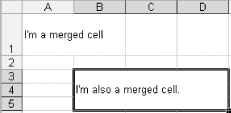
Joining multiple cells together removes the cells’ shared borders and creates one mega-sized cell. Usually, you’ll do this to accommodate a large amount of content that can’t fit in a single cell (like a long title that you want to display over every column). For example, if you merge cells A1 and B1, you’ll end up with a single cell named A1 that stretches over the full width of the A and B columns, as shown here.
To merge cells, select the cells you want to join, choose Format → Cells, and on the Alignment tab, turn on the “Merge cells” checkbox. There’s no limit to how many cells you can merge. (In fact, you can actually convert your entire worksheet into a single cell if you so desire.) And if you change your mind, don’t worry—you simply need to select the single merged cell, choose Format → Cells again, and clear the checkmark in the “Merge cells” checkbox to redraw the original cells.
Finally, the Alignment tab allows you to rotate content in a cell up to 180 degrees, as shown in Figure 4-9. You can set the number of degrees in the Orientation box on the right of the Alignment tab. Rotating cell content automatically changes the size of the cell. Usually, you’ll see it become narrower and taller to accommodate the rotated content.
As in almost any Windows program, you can customize the text in Excel, applying a dazzling assortment of colors and fancy typefaces. You can do everything from enlarging headings to shrinking footnotes. Other settings you can change include:
The font style. (For example, Arial, Times New Roman, or something a little more shocking, like Futura Extra Bold). Arial is the standard font for new worksheets.
The font size, in points. The default point size is 10, but you can choose anything from a minuscule 1-point to a monstrous 409-point. Excel automatically enlarges the row height to accommodate the font.
Various font attributes, like italics, underlining, and bold. Some fonts have complimentary italic and bold typefaces, while others don’t (in which case Windows will use its own algorithm to embolden or italicize the font).
The font color. This option controls the color of the text. (The next section (Section 4.2.3) covers how to change the color of the entire cell.)
To change font settings, first highlight the cells you want to format, choose Format → Cells, then click the Font tab (Figure 4-10). The Formatting toolbar also provides a number of shortcuts that let you quickly change certain font settings, including font, size, color, and attributes like boldface and italics. The Formatting toolbar sits in the row just under Excel’s main menu and is described in more detail in Section 4.3.1. (Truth be told, the formatting toolbar is way more convenient for setting fonts, because its drop-down menu shows a long list of font names, whereas the font list in the Format Cells dialog box is limited to showing an impossibly restrictive four fonts at a time. Scrolling through that cramped space is more than a little maddening.)
Note
No matter what font you apply, Excel, thankfully, always displays the cell contents in the Arial font in the Formula bar. That makes things easier if you happen to be working with cells that have been formatted to use graphically complex or large fonts.
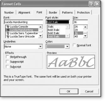
Figure 4-10. Here’s an example of what happens when you apply an exotic font through the Format Cells dialog box. Keep in mind that, when displaying data and especially numbers, sans-serif fonts are usually clearer and look more professional than serif fonts. (Serif fonts have little embellishments, like tiny curls, on the ends of the letters; sans-serif fonts don’t.) Arial, the default spreadsheet font, is a sans-serif font. The font used for the body text of this book, Adobe Minion, is clearly a serif font, which works best for large amounts of text.
Tip
The default font in an Excel worksheet is Arial but you can change this setting easily. To do so, select Tools → Options, and then click the General tab. Next to the “Standard font” label are two drop-down menus where you can set the standard font and font size. The font you choose won’t apply to existing worksheets, but Excel will use it every time you create a new worksheet.
Most fonts contain not only digits and the common letters of the alphabet, but also some special symbols that you can type directly on your keyboard. One example is the copyright symbol ©, which you can insert into a cell by entering the text (C), and letting AutoCorrect do its work. Other symbols, however, aren’t as readily available. One example is the special arrow character → . To use this symbol, you’ll need the help of the Wingdings font.
Wingdings is a special font included with Windows that’s made up entirely of symbols like arrows and icons, none of which are found in standard fonts. You can try and apply the Wingdings font on your own, but it won’t be easy, because you won’t know which character to press on your keyboard to get the symbol you want. A better choice is to use Excel’s Symbol dialog box. Simply follow these steps:
Choose Insert → Symbol from the menu.
The Symbol dialog box opens, as shown in Figure 4-11.
Choose the font that has the special character.
Excel selects the Wingdings font automatically—which is good news, because it has the most interesting symbols for you to use. In addition, you can find a few predefined special characters, like the copyright symbol, on the Special Characters tab of the Symbol dialog box.
Select the character in the character map, and then click Insert.
Alternatively, if you need to insert multiple special characters, just double-click each one; doing so inserts each symbol right next to each other in the same cell without having to close the window.
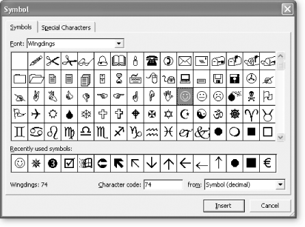
When Excel inserts a character from the Symbol dialog box, it doesn’t change the font for the cell. What you’ll actually end up with is a cell that has two fonts—one for the symbol character and one that’s used for the rest of your text. This works perfectly well, but it can cause some confusion. For example, if you apply a new font to the cell after inserting a special character, Excel adjusts the entire contents of the cell to use the new font, and your symbol will change into the corresponding character in the new font (which usually isn’t what you want). These problems can crop up any time you deal with a cell that has more than one font.
Note
If you look at the cell contents in the Formula bar, you’ll always see the cell data in the standard Arial font. That means, for example, that your Wingdings symbol won’t appear as the icon that shows up in your worksheet. Instead, you’ll see an ordinary letter or some type of extended non-English character, like æ.
The best way to call attention to important information isn’t to change fonts or alignment. Instead, place borders around key cells or groups of cells and use shading to highlight important columns and rows. Excel provides dozens of different ways to outline and highlight any selection of cells.
Once again, the trusty Format Cells dialog box is your control center. Just follow these steps:
Select the cells you want to fill or outline.
Your selected cells appear highlighted (see Figure 4-12).
Figure 4-12. You can remove a worksheet’s gridlines, as shown here, which is handy when you want to more easily see any custom borders you’ve added. Select Tools → Options from the menu, select the View tab, and then turn off the checkmark next to the Gridlines checkbox. (This affects only the current file, and won’t apply to new spreadsheets.)
Note
The Gridlines setting has no effect on whether or not Excel adds the worksheet gridlines to a printout. You can control whether your borders appear in printed versions of your worksheet through the Page Layout setting, as described on Section 6.2.2.4.
Select Format → Cells, or just right-click the selection, and choose Format Cells.
The Format Cells dialog box appears.
Head directly to the Border tab.
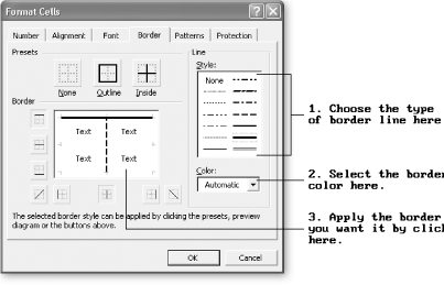
(If you don’t want to apply any borders, skip straight to step 4.) Applying a border is a multistep process (see Figure 4-13). Begin by choosing the line style you want (dotted, dashed, thick, double, and so on), followed by the color (Automatic picks black). Both these options are on the right side of the tab. Next, choose where your border lines are going to appear. The Border box (where the word “Text” appears four times) functions as a nifty interactive test canvas that shows you where your lines are going to appear. To make your selection you can either click one of the eight Border buttons (which contain a single bold horizontal, vertical, or diagonal line), or you can click directly inside the Border box. If you change your mind, clicking a border line will make it disappear.
For example, if you want to apply a border to the top of your selection, click the top of the Border box. If you want to apply a line between columns inside the collection, click between the cell columns in the Border box. The line appears indicating your selection.
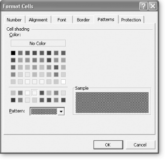
Here you can select the color and pattern of any shading you want to add to the cells in the selection (see Figure 4-14). Click the No Color box to clear any current color or pattern in the selected cells.
Figure 4-14. Adding a pattern to selected cells is simpler than choosing borders. All you need to do is select the color you want and optionally choose a pattern. The pattern is always drawn in black, and can include diagonal lines, a grid, dots, or the tight checkerboard shown in this figure. Generally, patterns obscure text, and you shouldn’t apply them to cells that have content. Fills tend to work better, provided you use light colors that will allow text or numbers to remain legible.
Click OK to apply your changes.
If you don’t like the modifications you’ve just applied, you can roll back time with a quick application of the Edit → Undo command.
You’ve now had a comprehensive tour of Excel’s formatting features. But of course, just because the features are there doesn’t mean they’re easy to use. Digging through the different options, and applying a full range of formatting choices can be a tedious task. Fortunately, Excel also includes a few timesavers that let you speed up many formatting tasks. The final few sections of this chapter introduce these features. You’ll see how to skip the Format Cells dialog box with a few toolbar tricks, how to copy and standardize formatting with Styles and the Format Painter, and how to add a little built-in graphical intelligence to your worksheet with conditional formatting.
GEM IN THE ROUGH: Your Favorite Colors
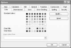
Excel gives you a fairly narrow set of color choices for fonts, borders, and fills, which you can find by choosing Tools → Options and then clicking the Colors tab. The 56 colored boxes there are you basic choices. You can, however, alter those. Select one of the color boxes, and then click the Modify button. You’ll see a more extensive dialog box that lets you pick an exact shade.
Bear in mind that you can’t tweak any of the colors while you’re formatting a cell. Instead, you need to set the color beforehand. Also, although Excel lets you modify colors, there’s no way to create extra colors in a worksheet.
Color settings are specific to a single workbook file. However, you can copy them from one file to another. Just open both workbooks at once, and then, in the workbook where you want to place the copied colors, choose Tools → Options. Click the color tab, and then, in the “Copy colors from” list, find the name of the workbook that has the colors you want to copy. Excel refreshes the set of colors immediately. You can also click Reset to return your color settings to Excel’s standard choices.
In order to control cell formatting, you need to jump between your worksheet and the Format Cells dialog box, which can be time-consuming. But what if there were a way to apply basic formatting without jumping to a new window? In fact, Excel provides a handy shortcut with its Formatting toolbar.
The Formatting toolbar can’t duplicate every feature in the Format Cells dialog box. However, it does let you apply the most common types of formatting with one or two quick clicks of the mouse.
Note
The Formatting toolbar is usually displayed at the top of the Excel window. If you’ve lost yours, just select View → Toolbars → Formatting from the menu.
Using the Formatting toolbar is similar to using the Format Cells dialog box. First, move to the cell you want to change, or select a group of cells. Then click the appropriate button in the toolbar to apply a new font, fill pattern, border, or cell value format. Figure 4-15 outlines your options.
But wait . . . there’s more! The Formatting toolbar also includes a few tools that aren’t available in the Format Cells dialog box: The ability to draw borders directly on the worksheet and a way to format individual characters. The next two sections show you how.
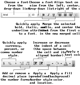
Figure 4-15. The Formatting toolbar provides one-stop shopping for a number of formatting options. When you use the font list, you’ll even see the name of the font displayed in its proper typeface (so the font entry “Times New Roman” is displayed using Times New Roman, which gives you a helpful preview).
The Borders button on the Formatting toolbar lets you quickly apply basic borders to the current selection. This is an ideal way to add a column divider or outline a group of cells with column headings. But what if you want to create more elaborate borders? There’s no need to head to the Format Cells dialog box if you don’t want to, because Excel gives you the ability to draw cell borders directly onto your worksheet. It works like this:
Click the drop-down arrow next to the Borders icon in the Formatting toolbar. Choose the last option in the menu, Draw Borders.
The Borders toolbar appears automatically, with the Draw Border icon already selected (see Figure 4-16).
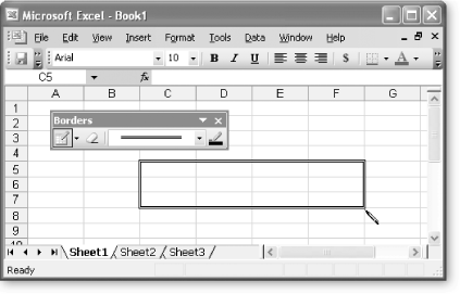
Figure 4-16. The Borders toolbar looks humble enough, but it packs a lot of power. Rather than allowing you to apply only preset border styles to the current selection, the Borders toolbar lets you draw directly onto your worksheet. To activate drawing mode, make sure you’ve selected the Draw Border icon on the left side of the toolbar. You can also choose a line style and color.
Choose a line style and color in the Borders toolbar.
The line and color options are similar to the Borders tab in the Format Cells dialog box.
Begin drawing your borders by single clicking on the lines between cells.
To draw a longer border, drag your pointer down through a range of cells. If you drag your pointer down and to the side, you’ll create an external border around a block of cells. Alternatively, you can choose to draw a border across a block of cells by changing the drawing mode. Click the drop-down arrow next to the Draw Border icon on the Borders toolbar, and choose Draw Border Grid (instead of the standard option, Draw Border). Now, when you drag the mouse over a rectangular region of cells, you’ll add border lines to all the cells you drag across.
If you want to erase a border, click the Erase icon on the Borders toolbar. The pointer changes to an eraser and you can click the border you want to remove.
To stop drawing, deselect the Draw Border icon on the Borders toolbar.
Even once you stop drawing borders, the Borders toolbar remains, ready for use. If you’re finished with it, you can hide it by selecting View → Toolbars → Borders, or click the X on the toolbar’s right side.
The Formatting toolbar lets you perform one task that isn’t possible with the Format Cells dialog box: applying formatting to just a part of a cell. For example, if a cell contains the text “New low price,” you could apply a new color or bold format to the word “low.”
To apply formatting to a portion of a cell, follow these steps:
Move to the appropriate cell, and put it into edit mode by pressing F2.
You can also put a cell into edit mode by double-clicking it, or by moving to it and clicking inside the text in the Formula bar.
Select the text you want to format.
You can select the text by highlighting it with the mouse or by holding down Shift while using the arrow keys to mark your selection.
Choose a font option from the toolbar.
You can change the size, the font, the color, or the bold, italic, or underline settings.
Note
Applying multiple types of text formatting to the same cell can get tricky. The Formula bar won’t show the difference, and, when you edit the cell, you might not end up entering text in the font you want. Also, be careful that you don’t apply new font formatting to the cell later; if you do, you’ll wipe out all the font information you’ve added to the cell.
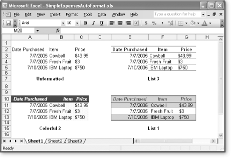
Although AutoFormat doesn’t automatically take care of all the formatting you may need to do on a spreadsheet, it does take a basic, unformatted table of information, and automatically apply a collection of borders, fills, and bold or italic formatting to highlight the table’s structure. Figure 4-17 shows some examples of AutoFormat at work.
To use AutoFormat, follow these steps:
Select the cells you want to AutoFormat.
In fact, you can move to any cell that’s within the cells you want to AutoFormat. AutoFormat can automatically detect which portion of a worksheet is filled with data—as long as there are no blank rows or columns within the data. If you have a table of data that includes blank rows or columns (for example, you’ve left a blank row between you’re heading and column titles), you’ll need to manually select the entire range of cells you want to AutoFormat before continuing.
Select Format → AutoFormat from the menu.
If you haven’t already manually selected your cells, AutoFormat starts by selecting all the cells it thinks you want to format. Then the AutoFormat window appears, displaying a list of preset format templates.
Figure 4-17. This worksheet shows the before and after effects of using Autoformat. The first table of data shows the data before it’s been formatted; the other three tables have been transformed using a variety of different AutoFormat templates.
Choose one of the format templates.
Each template presents a different collection of column, border, number, and text format settings. The templates have semi-descriptive names, like Accounting 1 and Classic 2. Click the template most closely matching the look you want. Unfortunately, you can’t create your own templates. But you can modify some of the settings in the existing templates, as shown in Figure 4-18. You can also adjust the format settings after you apply them using the Format Cells dialog box.
Click OK.
Excel applies the AutoFormat template to your data.
The Format Painter is a simple yet elegant tool that lets you copy all cell format settings—including fonts, colors, patterns, and borders—from one cell to another. (Apparently the Excel team decided that the more accurate label “Format Copier” wasn’t nearly as exciting as the name Format Painter.)
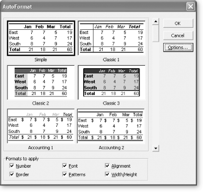
Figure 4-18. Each format template includes settings for number formats, fonts, alignment, borders, fill patterns, row height, and column width. Click the Options button if you want your chosen template to not include any of these individual settings. A new group of checkboxes will appear at the bottom of the AutoFormat window, and you can clear the checkboxes corresponding to the format options you don’t want to apply.
To use the Format Painter, follow these steps:
Move to a cell that has the formatting you want to copy.
You can use the Format Painter to copy formatting from either one cell or a whole group of cells. For example, you could copy the format from two cells that use two different fill colors, and paste that format to a whole range of new cells. These cells would alternate between the two fill colors. Although this is a powerful trick, in most cases it’s easiest to copy the format from a single cell.
Click the Format Painter button on the Standard toolbar (Figure 4-19), to switch into “format painting” mode.
The pointer changes so that it now includes a paintbrush icon, indicating Excel is ready to copy the format.
Click the cell where you want to apply the format.
The moment you release your mouse button, Excel applies the formatting and your pointer changes back to its normal appearance. If you want to copy the selected format to several cells at once, just drag to select a group of cells, rows, or columns, instead of clicking a single cell.
Figure 4-19. Oddly enough, the Format Painter appears on the Standard toolbar instead of the Formatting toolbar. You can recognize the icon because it looks like a paintbrush.
Excel doesn’t let you get too carried away with format painting—as soon as you copy the format to a new cell or selection, you exit format painting mode. If you want to copy the desired format to another cell, you have to backtrack to the cell that has your format, and start over again. However, there’s a neat trick you can use if you know you’re going to repeatedly apply the same format to a bunch of different cells. Instead of single-clicking the Format Painter button, double-click it. You’ll remain in format painting mode until you click the Format Painter button again to switch it off.
Note
The Format Painter is a good tool for quickly copying formatting, but it’s no match for another Excel feature called Styles. With Styles, you can define a group of formatting settings, and apply them wherever you need them. Best of all, if you change the style after you’ve created it, Excel automatically updates all cells that you’ve formatted using that style. Styles are described in the next section.
Styles let you create a customized combination of format settings, give it a name, and store it in a spreadsheet file. You can then apply these settings anywhere you need them.
Styles really shine in complex worksheets where you need to apply different formatting to different groups of cells. For example, say you’ve got a worksheet that’s tracking your company’s performance. You’re confident that most of the data is reliable, but there are a few rows that come from your notoriously overly optimistic sales department. To highlight these sales projections, you decide to use a combination of a bold font with a hot pink fill. And since these figures are estimated and aren’t highly precise, you decide to use a number format without decimal places and precede the number with a tilde (~), the universal symbol for “approximately right.”
You could implement all these changes manually. But that’ll take fourscore and seven years. Better to set up a style that includes all these settings and then apply it with a flick of the wrist whenever you need it. Styles are efficiency monsters in a few ways:
They let you reuse your formatting easily, just by applying the style.
They free you from worry about being inconsistent, because the style includes all the formatting you want.
Excel automatically saves styles with your spreadsheet file, and you can transfer styles from one workbook to another.
If you decide you need to change a style, it requires just a few mouse clicks. Then, Excel automatically adjusts every cell that uses your style.
What more could you want?
Begin by moving to a cell in your worksheet that has the formatting you want to use for your style.
The quickest way to create a new style is by using formatting you’ve already set up. However, you can also create a new style from scratch. In this case, you would simply move to a blank, unformatted cell in your worksheet.
Select Format → Style.
This action opens the Style dialog box, which provides a drop-down list of styles. Usually, the Normal style will be selected in this list, unless you’ve already applied a different style to the current cell.
Type a name for your new style into the “Style name” list box.
The text you type replaces the current selection. For example, if you want to create a new style for column titles, you might enter the style name ColumnTitle. Each style name needs to be unique in your spreadsheet file. Figure 4-20 shows a new style being created.
Click Add to create the new style.
Your style now exists and is based on the formatting settings of the current cell. The next step explains how to modify these settings.
Click Modify to specify the formatting options for the style.
When you click Modify, the familiar Format Cells dialog box appears. You can use this dialog box to change formatting just as if you were formatting an individual cell. Click OK to close the Format Cells dialog box when you’re finished.
Click OK to close the Style window.
You can return to the Style window at any time to modify existing styles, or delete them, using the Modify and Delete buttons.
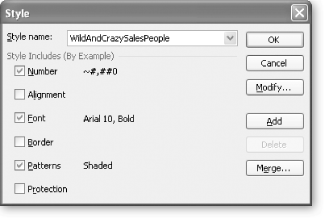
Figure 4-20. Here, a new style, WildAndCrazySalesPeople, is about to be created. This style defines a number format as well as alignment, font, border, and pattern settings. If you don’t want your style to include any of these settings, turn off the checkmark in the appropriate checkboxes. For example, if you want to create a style that applies a new font, fill, and border, but you want to keep the existing alignment and number format, turn off the Number and Alignment checkboxes. As a general rule, if you don’t need to explicitly set a specific style characteristic, turn off the corresponding checkmark.
Once you’ve created a style, applying it is just a matter of a few mouse clicks. Select the cell or cells you want to modify, choose Format → Style, choose your style from the list, and click OK. You’ll see the changes immediately.
Keep in mind that you can still modify the formatting of a cell after you’ve applied a style. But if you do find yourself overriding a style fairly frequently, and always in the same way, you probably need to modify the style. Either create more than one version of the same style, each with the appropriate settings, or clear some of the Style checkboxes so that your style won’t apply formatting settings that you commonly change.
Every worksheet also includes a basic set of default styles, which you can see in the Style window. These styles are:
Normal is the standard style that Excel applies to all cells in a new worksheet. It sets the number format to General and the font to 10-point Arial (unless you’ve changed the standard font). It also turns off shading and borders and sets the vertical alignment to Bottom and the horizontal alignment to General.
Comma changes the number format to Accounting, set to two decimal places. The Accounting format always uses a comma to separate each group of three digits (for example: 385,789).
Comma [0] changes the number format to Accounting but doesn’t include any decimal places.
Currency, oddly enough, doesn’t use the Currency number format. Instead, it changes the number format to Accounting, set to two decimal places and using the currency symbol defined in your regional settings (such as $) at the beginning of the number. The only difference between this choice and the Currency number format is that Excels lines up currency signs at the left side of the cell, and pads cell values with one space on the right.
Currency [0] changes the number format to Accounting, but doesn’t include any decimal places. It also uses a currency symbol (such as $).
Percent changes the number format to Percent and doesn’t include any decimal places.
With the exception of Normal, these styles apply only a single formatting characteristic: a number format. You’ll notice that none of the other style checkboxes are turned on. You can modify all of these styles, and you can remove any of them except for Normal.
Once you’ve created a few useful styles, you’ll probably want to reuse them in a variety of spreadsheet files. In order to do this, you need to copy the style information from one workbook to another. Excel makes this process fairly straightforward:
Open both files in Excel.
You’ll need both the source workbook (the one that has the styles you want to copy) and the destination workbook (the one where you want to copy the styles).
Go to the destination workbook.
Choose Format → Style.
The Style dialog box appears.
Click the Merge button.
The Merge Styles dialog box appears with a list of all files that you currently have open in Excel.
Select the file that has the styles you want to copy into your active workbook, and click OK.
If there are any files that have the same name, Excel prompts you with a warning message, informing you that it will overwrite the current styles with the styles you’re importing. Click OK to continue.
Click OK to close the Style dialog box.
You can now use the styles that you’ve imported. These styles are now an independent copy of the styles in the source workbook. If you change the styles in one workbook, the other workbook won’t be affected unless you import the changed styles into it.
Earlier in this chapter, you learned how to create custom format strings. Excel allows you to create up to three different format strings for the same cell. For example, you can define a format string for positive numbers, a format string for negative numbers, and another format string for zero values. Using this technique, you could create a worksheet that automatically highlights negative numbers in red lettering while leaving non-negative numbers in black. This trick saves you the trouble of having to manually find the offending cells and apply a different font color.
This ability to treat negative numbers differently from positive numbers is quite handy, but it’s obviously limited. For example, what if you want to flag extravagant expenses that top $100, or you want to flag a monthly sales total if it exceeds the previous month’s sales by 50%? Custom format strings can’t help you there, but Excel does provide another feature to fill in the gap: conditional formatting.
With conditional formatting, you set a condition that, if true, prompts Excel to apply additional formatting to a cell. This new formatting can change the text color or use any other formatting trick you’ve seen in this chapter, including modifying fill colors, borders, and fonts. Usually, conditional formatting is used as a way to automatically highlight something important in a spreadsheet.
To apply conditional formatting, follow these steps:
Select the cell you want to apply the conditional formatting to.
You can apply conditional formatting to any cell or combination of cells.
Select Format → Conditional Formatting.
The Conditional Formatting dialog box appears. It lets you set up to three conditions for a cell. When the window first appears, it shows only a single condition, which is usually all you need.
Using the list and text boxes, set the condition that Excel should evaluate.
The first drop-down list box allows you to choose whether you want to evaluate a formula (“Formula Is”) or examine the cell value (“Cell Value Is”). The simplest option is to examine the cell value. (Formulas are covered in detail starting in Chapter 7).
Using the second drop-down list box, choose the type of comparison you want to perform. You can choose to test whether the cell value equals a set number, is greater or less than a set number, or lies within some range of values.
Finally, enter the information that Excel should use for the comparison. For example, if you choose to perform a less-than comparison, type in the value that Excel should compare against. If you choose to test whether a cell is between certain values, enter both values in this range.
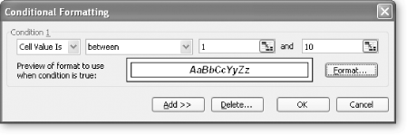
Figure 4-21 shows a completed Conditional Formatting dialog box.
Figure 4-21. In this example, the cell will contain italicized, bold text and will be surrounded by a black border—if the number in the cell is between 1 and 10.
Tip
Usually, conditional formatting compares a cell value to a fixed number or constant. However, you can also create conditions that compare the cell value to other cells in your worksheet. To take this step, select the text box where you’d enter the comparison number, and then click the worksheet to select the cell that Excel should use. Excel automatically inserts a cell reference (like $D$2 for cell D2) into the text box.
Click the Format button to set the formatting that Excel should apply if the condition is true.
An abbreviated version of the Format Cells dialog box appears featuring the Font, Border, and Patterns tab. Other settings, like the number format, can’t be applied conditionally, and so they won’t appear. You also can’t conditionally change the font (the Font tab only lets you control the Font style). However, aside from these limitations, the tabs are exactly the same as the ones you’re familiar with from the full-blown Format Cells dialog box (Figure 4-2).
Click OK to close the Format Cells dialog box.
In the Conditional Formatting window underneath your condition, you’ll see a preview of the formatting choices you made.
If you want to add a second or third condition, click Add, and return to step 3.
Excel evaluates each condition separately and applies the appropriate formatting.
You can also click Delete to remove conditions. Excel will display a dialog box asking which conditions you want to remove. You can then place a checkmark next to the appropriate condition and click OK.
Click OK.
As soon as you click OK, Excel evaluates the conditions and adjusts the formatting as needed. Every time you open your spreadsheet, or change the value in the conditional cell, Excel evaluates the condition.
Note
Conditional formatting is like any other type of formatting in Excel. To remove conditional formatting, select the cell and choose Edit → Clear → Formats. You can also copy conditional formatting from one cell to another using the Format Painter (although you can’t make conditional formatting part of a style).
Get Excel 2003: The Missing Manual now with the O’Reilly learning platform.
O’Reilly members experience books, live events, courses curated by job role, and more from O’Reilly and nearly 200 top publishers.

