3.6. Frequential characterization of a continuous-time system
3.6.1. First and second order filters
3.6.1.1. 1st order system
Let us look at a physical system regulated by a linear differential equation of the 1st order, as is usually the case with RC and LR type filters:
![]()
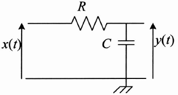
Figure 3.23. RC filter
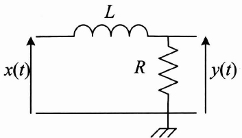
Figure 3.24. LR filter
The transmittance of the system, i.e. ![]() , where Y(s) designates the Laplace transform1 of y(t) and is expressed by:
, where Y(s) designates the Laplace transform1 of y(t) and is expressed by:
![]()
In taking s = jω where ω = 2πf designates the angular frequency, we obtain:

where K is called the static gain.
With RC and LR filters, the time constant is worth, respectively, τ = RC and ![]() and K = 1.
and K = 1.
We characterize the system by its impulse response or its indicial response. When x(t) = δ(t), X(s) = 1.
From there:
and if we refer to a Laplace transform table, ...
Get Digital Filters Design for Signal and Image Processing now with the O’Reilly learning platform.
O’Reilly members experience books, live events, courses curated by job role, and more from O’Reilly and nearly 200 top publishers.

