Chapter 1. Introduction
This book is about doing data science at the command line. Our aim is to make you a more efficient and productive data scientist by teaching you how to leverage the power of the command line.
Having both the terms “data science” and “command line” in the title requires an explanation. How can a technology that’s over 40 years old1 be of any use to a field that’s only a few years young?
Today, data scientists can choose from an overwhelming collection of exciting technologies and programming languages. Python, R, Hadoop, Julia, Pig, Hive, and Spark are but a few examples. You may already have experience in one or more of these. If so, then why should you still care about the command line for doing data science? What does the command line have to offer that these other technologies and programming languages do not?
These are all valid questions. This first chapter will answer these questions as follows. First, we provide a practical definition of data science that will act as the backbone of this book. Second, we’ll list five important advantages of the command line. Third, we demonstrate the power and flexibility of the command line through a real-world use case. By the end of this chapter we hope to have convinced you that the command line is indeed worth learning for doing data science.
Overview
In this chapter, you’ll learn:
-
A practical definition of data science
-
What the command line is exactly and how you can use it
-
Why the command line is a wonderful environment for doing data science
Data Science Is OSEMN
The field of data science is still in its infancy, and as such, there exist various definitions of what it encompasses. Throughout this book we employ a very practical definition by Mason & Wiggins (2010). They define data science according to the following five steps: (1) obtaining data, (2) scrubbing data, (3) exploring data, (4) modeling data, and (5) interpreting data. Together, these steps form the OSEMN model (which is pronounced as awesome). This definition serves as the backbone of this book because each step, (except step 5, interpreting data) has its own chapter. The following five subsections explain what each step entails.
Note
Although the five steps are discussed in a linear and incremental fashion, in practice it is very common to move back and forth between them or to perform multiple steps at the same time. Doing data science is an iterative and nonlinear process. For example, once you have modeled your data, and you look at the results, you may decide to go back to the scrubbing step to adjust the features of the data set.Obtaining Data
Without any data, there is little data science you can do. So the first step is to obtain data. Unless you are fortunate enough to already possess data, you may need to do one or more of the following:
-
Download data from another location (e.g., a web page or server)
-
Query data from a database or API (e.g., MySQL or Twitter)
-
Extract data from another file (e.g., an HTML file or spreadsheet)
-
Generate data yourself (e.g., reading sensors or taking surveys)
In Chapter 3, we discuss several methods for obtaining data using the command line. The obtained data will most likely be in either plain text, CSV, JSON, or HTML/XML format. The next step is to scrub this data.
Scrubbing Data
It is not uncommon that the obtained data has missing values, inconsistencies, errors, weird characters, or uninteresting columns. In that case, you have to scrub, or clean, the data before you can do anything interesting with it. Common scrubbing operations include:
-
Filtering lines
-
Extracting certain columns
-
Replacing values
-
Extracting words
-
Handling missing values
-
Converting data from one format to another
While we data scientists love to create exciting data visualizations and insightful models (steps 3 and 4), usually much effort goes into obtaining and scrubbing the required data first (steps 1 and 2). In “Data Jujitsu,” DJ Patil states that “80% of the work in any data project is in cleaning the data” (2012). In Chapter 5, we demonstrate how the command line can help accomplish such data scrubbing operations.
Exploring Data
Once you have scrubbed your data, you are ready to explore it. This is where it gets interesting, because here you will get really into your data. In Chapter 7, we show you how the command line can be used to:
-
Look at your data.
-
Derive statistics from your data.
-
Create interesting visualizations.
Command-line tools introduced in Chapter 7 include csvstat (Groskopf, 2014), feedgnuplot (Kogan, 2014), and Rio (Janssens, 2014).
Modeling Data
If you want to explain the data or predict what will happen, you probably want to create a statistical model of your data. Techniques to create a model include clustering, classification, regression, and dimensionality reduction. The command line is not suitable for implementing a new model from scratch. It is, however, very useful to be able to build a model from the command line. In Chapter 9, we will introduce several command-line tools that either build a model locally or employ an API to perform the computation in the cloud.
Interpreting Data
The final and perhaps most important step in the OSEMN model is interpreting data. This step involves:
-
Drawing conclusions from your data
-
Evaluating what your results mean
-
Communicating your result
To be honest, the computer is of little use here, and the command line does not really come into play at this stage. Once you have reached this step, it is up to you. This is the only step in the OSEMN model that does not have its own chapter. Instead, we kindly refer you to Thinking with Data by Max Shron (O’Reilly, 2014).
Intermezzo Chapters
In between the chapters that cover the OSEMN steps, there are three intermezzo chapters. Each intermezzo chapter discusses a more general topic concerning data science, and how the command line is employed for that. These topics are applicable to any step in the data science process.
In Chapter 4, we discuss how to create reusable tools for the command line. These personal tools can come from both long commands that you have typed on the command line, or from existing code that you have written in, say, Python or R. Being able to create your own tools allows you to become more efficient and productive.
Because the command line is an interactive environment for doing data science, it can become challenging to keep track of your workflow. In Chapter 6, we demonstrate a command-line tool called Drake (Factual, 2014), which allows you to define your data science workflow in terms of tasks and the dependencies between them. This tool increases the reproducibility of your workflow, not only for you but also for your colleagues and peers.
In Chapter 8, we explain how your commands and tools can be sped up by running them in parallel. Using a command-line tool called GNU Parallel (Tange, 2014), we can apply command-line tools to very large data sets and run them on multiple cores and remote machines.
What Is the Command Line?
Before we discuss why you should use the command line for data science, let’s take a peek at what the command line actually looks like (it may already be familiar to you). Figures 1-1 and 1-2 show a screenshot of the command line as it appears by default on Mac OS X and Ubuntu, respectively. Ubuntu is a particular distribution of GNU/Linux, which we’ll be assuming throughout the book.
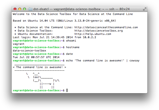
Figure 1-1. Command line on Mac OS X
The window shown in the two screenshots is called the terminal. This is the program that enables you to interact with the shell. It is the shell that executes the commands we type in. (On both Ubuntu and Mac OS X, the default shell is Bash.)
Note
We’re not showing the Microsoft Windows command line (also known as the Command Prompt or PowerShell), because it’s fundamentally different and incompatible with the commands presented in this book. The good news is that you can install the Data Science Toolbox on Microsoft Windows, so that you’re still able to follow along. How to install the Data Science Toolbox is explained in Chapter 2.Typing commands is a very different way of interacting with your computer than through a graphical user interface. If you are mostly used to processing data in, say, Microsoft Excel, then this approach may seem intimidating at first. Don’t be afraid. Trust us when we say that you’ll get used to working at the command line very quickly.
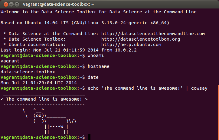
Figure 1-2. Command line on Ubuntu
In this book, the commands that we type in, and the output that they generate, is displayed as text. For example, the contents of the terminal (after the welcome message) in the two screenshots would look like this:
$ whoami
vagrant
$ hostname
data-science-toolbox
$ date
Tue Jul 22 02:52:09 UTC 2014
$ echo 'The command line is awesome!' | cowsay
 ______________________________
< The command line is awesome! >
 ------------------------------
        \   ^__^
         \  (oo)\_______
            (__)\       )\/\
                ||----w |
                ||     ||
You’ll also notice that each command is preceded with a dollar sign ($). This is called the prompt. The prompt in the two screenshots showed more information, namely the username (vagrant), the hostname (data-science-toolbox), and the current working directory (~). It’s a convention to show only a dollar sign in examples, because the prompt (1) can change during a session (when you go to a different directory), (2) can be customized by the user (e.g., it can also show the time or the current git (Torvalds & Hamano, 2014) branch you’re working on), and (3) is irrelevant for the commands themselves.
In the next chapter we’ll explain much more about essential command-line concepts. Now it’s time to first explain why you should learn to use the command line for doing data science.
Why Data Science at the Command Line?
The command line has many great advantages that can really make you a more an efficient and productive data scientist. Roughly grouping the advantages, the command line is: agile, augmenting, scalable, extensible, and ubiquitous. We elaborate on each advantage below.
The Command Line Is Agile
The first advantage of the command line is that it allows you to be agile. Data science has a very interactive and exploratory nature, and the environment that you work in needs to allow for that. The command line achieves this by two means.
First, the command line provides a so-called read-eval-print-loop (REPL). This means that you type in a command, press <Enter>, and the command is evaluated immediately. A REPL is often much more convenient for doing data science than the edit-compile-run-debug cycle associated with scripts, large programs, and, say, Hadoop jobs. Your commands are executed immediately, may be stopped at will, and can be changed quickly. This short iteration cycle really allows you to play with your data.
Second, the command line is very close to the filesystem. Because data is the main ingredient for doing data science, it is important to be able to easily work with the files that contain your data set. The command line offers many convenient tools for this.
The Command Line Is Augmenting
Whatever technology your data science workflow currently includes (whether it’s R, IPython, or Hadoop), you should know that we’re not suggesting you abandon that workflow. Instead, the command line is presented here as an augmenting technology that amplifies the technologies you’re currently employing.
The command line integrates well with other technologies. On the one hand, you can often employ the command line from your own environment. Python and R, for instance, allow you to run command-line tools and capture their output. On the other hand, you can turn your code (e.g., a Python or R function that you have already written) into a command-line tool. We will cover this extensively in Chapter 4. Moreover, the command line can easily cooperate with various databases and file types such as Microsoft Excel.
In the end, every technology has its advantages and disadvantages (including the command line), so it’s good to know several and use whichever is most appropriate for the task at hand. Sometimes that means using R, sometimes the command line, and sometimes even pen and paper. By the end of this book, you’ll have a solid understanding of when you could use the command line, and when you’re better off continuing with your favorite programming language or statistical computing environment.
The Command Line Is Scalable
Working on the command line is very different from using a graphical user interface (GUI). On the command line you do things by typing, whereas with a GUI, you do things by pointing and clicking with a mouse.
Everything that you type manually on the command line, can also be automated through scripts and tools. This makes it very easy to re-run your commands in case you made a mistake, when the data set changed, or because your colleague wants to perform the same analysis. Moreover, your commands can be run at specific intervals, on a remote server, and in parallel on many chunks of data (more on that in Chapter 8).
Because the command line is automatable, it becomes scalable and repeatable. It is not straightforward to automate pointing and clicking, which makes a GUI a less suitable environment for doing scalable and repeatable data science.
The Command Line Is Extensible
The command line itself was invented over 40 years ago. Its core functionality has largely remained unchanged, but the tools, which are the workhorses of the command line, are being developed on a daily basis.
The command line itself is language agnostic. This allows the command-line tools to be written in many different programming languages. The open source community is producing many free and high-quality command-line tools that we can use for data science.
These command-line tools can work together, which makes the command line very flexible. You can also create your own tools, allowing you to extend the effective functionality of the command line.
The Command Line Is Ubiquitous
Because the command line comes with any Unix-like operating system, including Ubuntu and Mac OS X, it can be found on many computers. According to an article on Top 500 Supercomputer Sites, 95% of the top 500 supercomputers are running GNU/Linux. So, if you ever get your hands on one of those supercomputers (or if you ever find yourself in Jurassic Park with the door locks not working), you better know your way around the command line!
But GNU/Linux doesn’t only run on supercomputers. It also runs on servers, laptops, and embedded systems. These days, many companies offer cloud computing, where you can easily launch new machines on the fly. If you ever log in to such a machine (or a server in general), there’s a good chance that you’ll arrive at the command line.
Besides mentioning that the command line is available in a lot of places, it is also important to note that the command line is not a hype. This technology has been around for more than four decades, and we’re personally convinced that it’s here to stay for another four. Learning how to use the command line (for data science) is therefore a worthwhile investment.
A Real-World Use Case
In the previous sections, we’ve given you a definition of data science and explained to you why the command line can be a great environment for doing data science. Now it’s time to demonstrate the power and flexibility of the command line through a real-world use case. We’ll go pretty fast, so don’t worry if some things don’t make sense yet.
Personally, we never seem to remember when Fashion Week is happening in New York. We know it’s held twice a year, but every time it comes as a surprise! In this section we’ll consult the wonderful web API of The New York Times to figure out when it’s being held. Once you have obtained your own API keys on the developer website, you’ll be able to, for example, search for articles, get the list of best sellers, and see a list of events.
The particular API endpoint that we’re going to query is the article search one. We expect that a spike in the amount of coverage in The New York Times about New York Fashion Week indicates whether it’s happening. The results from the API are paginated, which means that we have to execute the same query multiple times but with a different page number. (It’s like clicking Next on a search engine.) This is where GNU Parallel (Tange, 2014) comes in handy because it can act as a for loop. The entire command looks as follows (don’t worry about all the command-line arguments given to parallel; we’re going to discuss this in great detail in Chapter 8):
$ cd ~/book/ch01/data
$ parallel -j1 --progress --delay 0.1 --results results "curl -sL "\
> "'http://api.nytimes.com/svc/search/v2/articlesearch.json?q=New+York+'"\
> "'Fashion+Week&begin_date={1}0101&end_date={1}1231&page={2}&api-key='"\
> "'<your-api-key>'" ::: {2009..2013} ::: {0..99} > /dev/null

Computers / CPU cores / Max jobs to run
1:local / 4 / 1

Computer:jobs running/jobs completed/%of started jobs/Average seconds to
complete
local:1/9/100%/0.4s
Basically, we’re performing the same query for years 2009-2014. The API only allows up to 100 pages (starting at 0) per query, so we’re generating 100 numbers using brace expansion. These numbers are used by the page parameter in the query. We’re searching for articles in 2013 that contain the search term New+York+Fashion+Week. Because the API has certain limits, we ensure that there’s only one request at a time, with a one-second delay between them. Make sure that you replace <your-api-key> with your own API key for the article search endpoint.
Each request returns 10 articles, so that’s 1000 articles in total. These are sorted by page views, so this should give us a good estimate of the coverage. The results are in JSON format, which we store in the results directory. The command-line tool tree (Baker, 2014) gives an overview of how the subdirectories are structured:
$ tree results | head
results
└── 1
    ├── 2009
    │   └── 2
    │       ├── 0
    │       │   ├── stderr
    │       │   └── stdout
    │       ├── 1
    │       │   ├── stderr
    │       │   └── stdout
We can combine and process the results using cat (Granlund & Stallman, 2012), jq (Dolan, 2014), and json2csv (Czebotar, 2014):
$ cat results/1/*/2/*/stdout |> jq -c '.response.docs[] | {date: .pub_date, type: .document_type, '\
> 'title: .headline.main }' | json2csv -p -k date,type,title > fashion.csv
Let’s break down this command:
-
We combine the output of each of the 500
paralleljobs (or API requests). -
We use
jqto extract the publication date, the document type, and the headline of each article. 
-
We convert the JSON data to CSV using
json2csvand store it as fashion.csv.
With wc -l (Rubin & MacKenzie, 2012), we find out that this data set contains 4,855 articles (and not 5,000 because we probably retrieved everything from 2009):
$ wc -l fashion.csv
4856 fashion.csv
Let’s inspect the first 10 articles to verify that we have succeeded in obtaining the data. Note that we’re applying cols (Janssens, 2014) and cut (Ihnat, MacKenzie, & Meyering, 2012) to the date column in order to leave out the time and time zone information in the table:
$ < fashion.csv cols -c date cut -dT -f1 | head | csvlook
|-------------+------------+-----------------------------------------|
|  date       | type       | title                                   |
|-------------+------------+-----------------------------------------|
|  2009-02-15 | multimedia | Michael Kors                            |
|  2009-02-20 | multimedia | Recap: Fall Fashion Week, New York      |
|  2009-09-17 | multimedia | UrbanEye: Backstage at Marc Jacobs      |
|  2009-02-16 | multimedia | Bill Cunningham on N.Y. Fashion Week    |
|  2009-02-12 | multimedia | Alexander Wang                          |
|  2009-09-17 | multimedia | Fashion Week Spring 2010                |
|  2009-09-11 | multimedia | Of Color | Diversity Beyond the Runway  |
|  2009-09-14 | multimedia | A Designer Reinvents Himself            |
|  2009-09-12 | multimedia | On the Street | Catwalk                 |
|-------------+------------+-----------------------------------------|
That seems to have worked! In order to gain any insight, we’d better visualize the data. Figure 1-3 contains a line graph created with R (R Foundation for Statistical Computing, 2014), Rio (Janssens, 2014), and ggplot2 (Wickham, 2009).
$ < fashion.csv Rio -ge 'g + geom_freqpoly(aes(as.Date(date), color=type), '\
> 'binwidth=7) + scale_x_date() + labs(x="date", title="Coverage of New York'\
> ' Fashion Week in New York Times")' | display
By looking at the line graph, we can infer that New York Fashion Week happens two times per year. And now we know when: once in February and once in September. Let’s hope that it’s going to be the same this year so that we can prepare ourselves! In any case, we hope that with this example, we’ve shown that The New York Times API is an interesting source of data. More importantly, we hope that we’ve convinced you that the command line can be a very powerful approach for doing data science.
In this section, we’ve peeked at some important concepts and some exciting command-line tools. Don’t worry if some things don’t make sense yet. Most of the concepts will be discussed in Chapter 2, and in the subsequent chapters we’ll go into more detail for all the command-line tools used in this section.
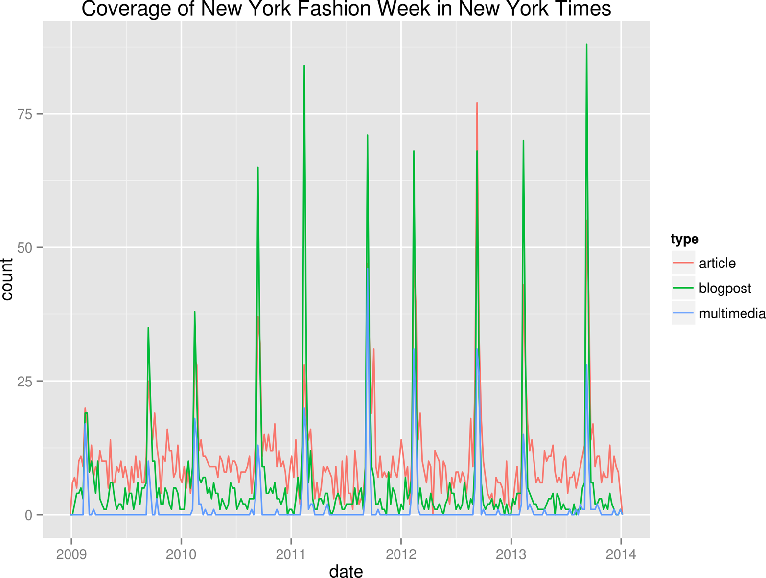
Figure 1-3. Coverage of New York Fashion Week in The New York Times
Further Reading
-
Mason, H., & Wiggins, C. H. (2010). A Taxonomy of Data Science. Retrieved May 10, 2014, from http://www.dataists.com/2010/09/a-taxonomy-of-data-science.
-
Patil, D (2012). Data Jujitsu. O’Reilly Media.
-
O’Neil, C., & Schutt, R. (2013). Doing Data Science. O’Reilly Media.
-
Shron, M. (2014). Thinking with Data. O’Reilly Media.
1 The development of the UNIX operating system started back in 1969. It featured a command line since the beginning, and the important concept of pipes was added in 1973.
Get Data Science at the Command Line now with the O’Reilly learning platform.
O’Reilly members experience books, live events, courses curated by job role, and more from O’Reilly and nearly 200 top publishers.

