Analysis of Financial Time Series, Third Edition

4.5 Application

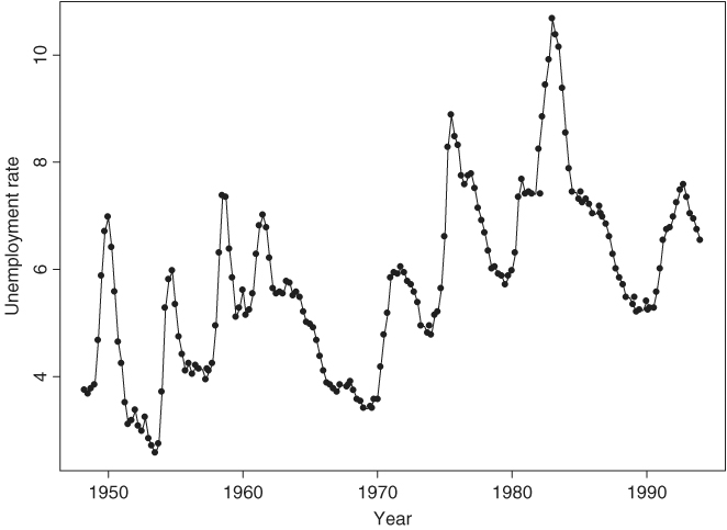
In this section, we illustrate nonlinear time series models by analyzing the quarterly U.S. civilian unemployment rate, seasonally adjusted, from 1948 to 1993. This series was analyzed in detail by Montgomery et al. (1998). We repeat some of the analyses here using nonlinear models. Figure 4.11 shows the time plot of the data. Well-known characteristics of the series include that (a) it tends to move countercyclically with U.S. business cycles, and (b) the rate rises quickly but decays slowly. The latter characteristic suggests that the dynamic structure of the series is nonlinear.

Figure 4.11 Time plot of U.S. quarterly unemployment rate, seasonally adjusted, from 1948 to 1993.

Denote the series by xt and let Δxt = xt − xt−1 be the change in unemployment rate. The linear model

4.52

was built by Montgomery et al. (1998), where the standard errors of the three coefficients are 0.11, 0.06, and 0.07, respectively. This is a seasonal model even though the data were seasonally adjusted. It indicates that the seasonal adjustment procedure used did not successfully remove the seasonality. This model is used as a benchmark model for forecasting comparison.

To test for nonlinearity, we apply some of the nonlinearity tests of Section 4.2 with an AR(5) model for the differenced ...