18.7 DESIGN 2: DESIGN SPACE EXPLORATION WHEN s2 = [1 0]
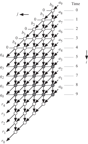
Figure 18.4 shows the DAG for the polynomial division algorithm based on our timing function choice s2. We note from the figure that the signals corresponding to the coefficients of B and the intermediate partial remainders corresponding to R and Q are all pipelined, as indicated by the arrows connecting the nodes. However, the estimated q output is broadcast among the nodes, as indicated by the horizontal lines without arrows. There are three simple projection vectors such that all of them satisfy Eq. 18.21 for the scheduling function in Eq. 18.18. The three projection vectors will produce three designs:
(18.31)
![]()
(18.32)
![]()
(18.33)
![]()
Figure 18.4 DAG for polynomial division algorithm when s2 = [1 0], n = 9, and m = 5.
The corresponding projection matrices are
(18.34)
![]()
(18.35)
![]()
(18.36)
Our multithreaded design space ...
Get Algorithms and Parallel Computing now with the O’Reilly learning platform.
O’Reilly members experience books, live events, courses curated by job role, and more from O’Reilly and nearly 200 top publishers.

