15.8 DESIGN 3: DESIGN SPACE EXPLORATION WHEN s = [1 0]t
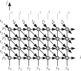
The dependence graph of Fig. 15.1 is transformed to the DAG in Fig. 15.11, which is associated with s = [1 0]t. The equitemporal planes are shown by the gray lines and the execution order is indicated by the gray numbers. We note that the variables P and T are pipelined between tasks, while variable Y is broadcast among tasks lying in the same equitemporal planes.
Figure 15.11 DAG for Design 3 when n = 10 and m = 4.
There are three simple projection vectors such that all of them satisfy Eq. 15.12 for the scheduling function. The three projection vectors are
(15.29)
![]()
(15.30)
![]()
(15.31)
![]()
Our multithreading design space now allows for three configurations for each projection vector for the chosen timing function.
15.8.1 Design 3.a: Using s = [1 0]t and da = [1 0]t
The ![]() corresponding to Design 3.a is drawn in Fig. 15.12 for the case when n = 10 and m = 4. Task Tj stores only the value pj, which can be stored in a register similar ...
corresponding to Design 3.a is drawn in Fig. 15.12 for the case when n = 10 and m = 4. Task Tj stores only the value pj, which can be stored in a register similar ...
Get Algorithms and Parallel Computing now with the O’Reilly learning platform.
O’Reilly members experience books, live events, courses curated by job role, and more from O’Reilly and nearly 200 top publishers.

