Think Stats, 2nd Edition

Chapter 4. Cumulative Distribution Functions

The code for this chapter is in cumulative.py. For information about downloading and working with this code, see Using the Code.

The Limits of PMFs

PMFs work well if the number of values is small. But as the number of values increases, the probability associated with each value gets smaller and the effect of random noise increases.

For example, we might be interested in the distribution of birth weights. In the NSFG data, the variable totalwgt_lb records weight at birth in pounds. Figure 4-1 shows the PMF of these values for first babies and others.

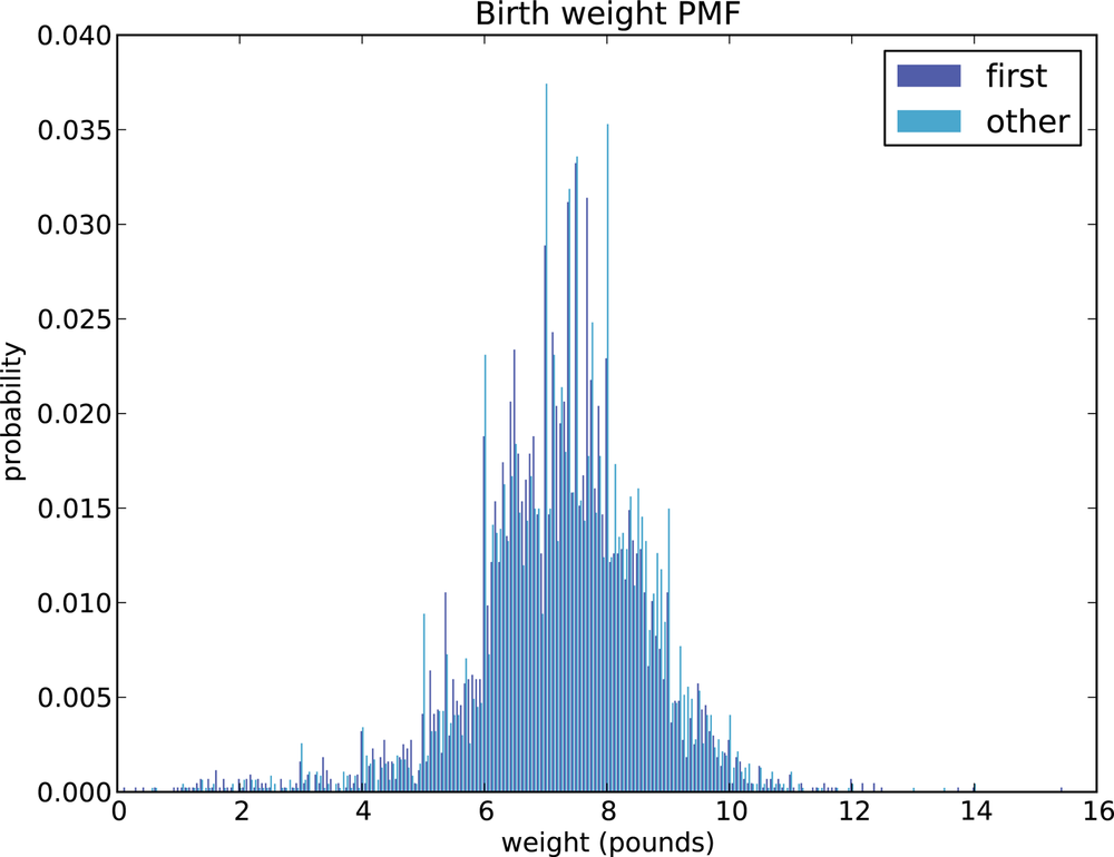
Figure 4-1. PMF of birth weights showing a limitation of PMFs: they are hard to compare visually

Overall, these distributions resemble the bell shape of a normal distribution, with many values near the mean and a few values much higher and lower.

But parts of this figure are hard to interpret. There are many spikes and valleys, and some apparent differences between the distributions. It is hard to tell which of these features are meaningful. Also, it is hard to see overall patterns; for example, which distribution do you think has the higher mean?

These problems can be mitigated by binning the data; that is, dividing the range of values into non-overlapping intervals and counting the number of values in each bin. Binning can be useful, but it is tricky to get the size of the bins right. If they are big enough to smooth out noise, they might also smooth out useful information.

An alternative that avoids these problems is the cumulative distribution function (CDF), which is the subject of this chapter. But before I can explain CDFs, I have to explain percentiles.

Percentiles

If you have taken a standardized test, you probably got your results in the form of a raw score and a percentile rank. In this context, the percentile rank is the fraction of people who scored lower than you (or the same). So if you are “in the 90th percentile,” you did as well as or better than 90% of the people who took the exam.

Here’s how you could compute the percentile rank of a value, your_score, relative to the values in the sequence scores:

def PercentileRank(scores, your_score):
    count = 0
    for score in scores:
        if score <= your_score:
            count += 1

    percentile_rank = 100.0 * count / len(scores)
    return percentile_rank

As an example, if the scores in the sequence were 55, 66, 77, 88 and 99, and you got the 88, then your percentile rank would be 100 * 4 / 5 which is 80.

If you are given a value, it is easy to find its percentile rank; going the other way is slightly harder. If you are given a percentile rank and you want to find the corresponding value, one option is to sort the values and search for the one you want:

def Percentile(scores, percentile_rank):
    scores.sort()
    for score in scores:
        if PercentileRank(scores, score) >= percentile_rank:
            return score

The result of this calculation is a percentile. For example, the 50th percentile is the value with percentile rank 50. In the distribution of exam scores, the 50th percentile is 77.

This implementation of Percentile is not efficient. A better approach is to use the percentile rank to compute the index of the corresponding percentile:

def Percentile2(scores, percentile_rank):
    scores.sort()
    index = percentile_rank * (len(scores)-1) / 100
    return scores[index]

The difference between “percentile” and “percentile rank” can be confusing, and people do not always use the terms precisely. To summarize, PercentileRank takes a value and computes its percentile rank in a set of values; Percentile takes a percentile rank and computes the corresponding value.

CDFs

Now that we understand percentiles and percentile ranks, we are ready to tackle the cumulative distribution function (CDF). The CDF is the function that maps from a value to its percentile rank.

The CDF is a function of x, where x is any value that might appear in the distribution. To evaluate for a particular value of x, we compute the fraction of values in the distribution less than or equal to x.

Here’s what that looks like as a function that takes a sequence, t, and a value, x:

def EvalCdf(t, x):
    count = 0.0
    for value in t:
        if value <= x:
            count += 1

    prob = count / len(t)
    return prob

This function is almost identical to PercentileRank, except that the result is a probability in the range 0–1 rather than a percentile rank in the range 0–100.

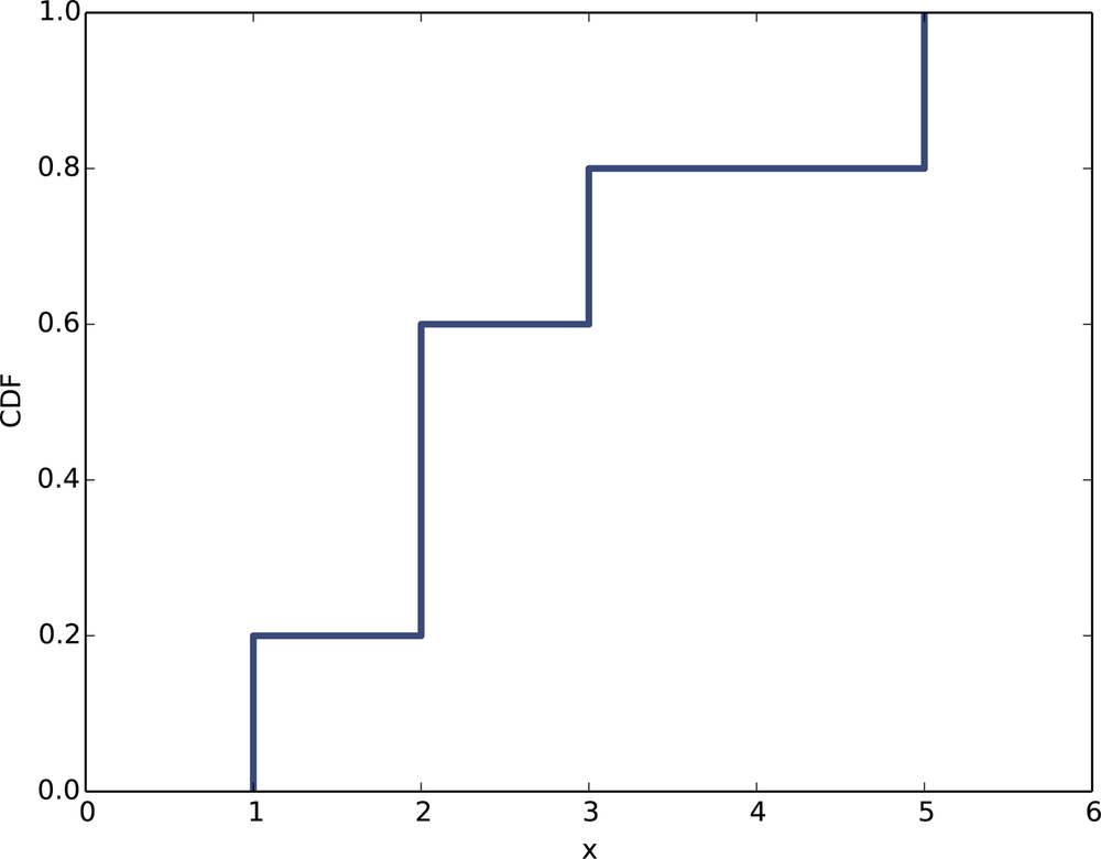
As an example, suppose we collect a sample with the values [1, 2, 2, 3, 5]. Here are some values from its CDF:

We can evaluate the CDF for any value of x, not just values that appear in the sample. If x is less than the smallest value in the sample, is 0. If x is greater than the largest value, is 1.

Figure 4-2 is a graphical representation of this CDF. The CDF of a sample is a step function.

Figure 4-2. Example of a CDF

Representing CDFs

thinkstats2 provides a class named Cdf that represents CDFs. The fundamental methods Cdf provides are:

Prob(x): Given a value x, computes the probability . The bracket operator is equivalent to Prob.
Value(p): Given a probability p, computes the corresponding value, x; that is, the inverse CDF of p.

The Cdf constructor can take as an argument a list of values, a pandas Series, a Hist, Pmf, or another Cdf. The following code makes a Cdf for the distribution of pregnancy lengths in the NSFG:

    live, firsts, others = first.MakeFrames()
    cdf = thinkstats2.Cdf(live.prglngth, label='prglngth')

thinkplot provides a function named Cdf that plots Cdfs as lines:

    thinkplot.Cdf(cdf)
    thinkplot.Show(xlabel='weeks', ylabel='CDF')

Figure 4-3 shows the result. One way to read a CDF is to look up percentiles. For example, it looks like about 10% of pregnancies are shorter than 36 weeks, and about 90% are shorter than 41 weeks. The CDF also provides a visual representation of the shape of the distribution. Common values appear as steep or vertical sections of the CDF; in this example, the mode at 39 weeks is apparent. There are few values below 30 weeks, so the CDF in this range is flat.

Figure 4-3. CDF of pregnancy length

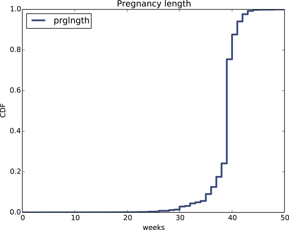
It takes some time to get used to CDFs, but once you do, I think you will find that they show more information, more clearly, than PMFs.

Comparing CDFs

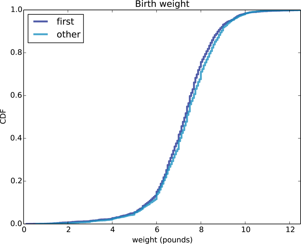
CDFs are especially useful for comparing distributions. For example, here is the code that plots the CDF of birth weights for first babies and others.

    first_cdf = thinkstats2.Cdf(firsts.totalwgt_lb, label='first')
    other_cdf = thinkstats2.Cdf(others.totalwgt_lb, label='other')

    thinkplot.PrePlot(2)
    thinkplot.Cdfs([first_cdf, other_cdf])
    thinkplot.Show(xlabel='weight (pounds)', ylabel='CDF')

Figure 4-4 shows the result. Compared to Figure 4-1, this figure makes the shape of the distributions, and the differences between them, much clearer. We can see that first babies are slightly lighter throughout the distribution, with a larger discrepancy above the mean.

Figure 4-4. CDF of birth weights for first babies and others

Percentile-Based Statistics

Once you have computed a CDF, it is easy to compute percentiles and percentile ranks. The Cdf class provides these two methods:

PercentileRank(x): Given a value x, computes its percentile rank, .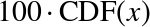
Percentile(p): Given a percentile rank rank, computes the corresponding value, x. Equivalent to Value(p/100).

Percentile can be used to compute percentile-based summary statistics. For example, the 50th percentile is the value that divides the distribution in half, also known as the median. Like the mean, the median is a measure of the central tendency of a distribution.

Actually, there are several definitions of “median,” each with different properties. But Percentile(50) is simple and efficient to compute.

Another percentile-based statistic is the interquartile range (IQR), which is a measure of the spread of a distribution. The IQR is the difference between the 75th and 25th percentiles.

More generally, percentiles are often used to summarize the shape of a distribution. For example, the distribution of income is often reported in “quintiles”; that is, it is split at the 20th, 40th, 60th and 80th percentiles. Other distributions are divided into 10 “deciles”. Statistics like these that represent equally spaced points in a CDF are called quantiles.

Random Numbers

Suppose we choose a random sample from the population of live births and look up the percentile rank of their birth weights. Now suppose we compute the CDF of the percentile ranks. What do you think the distribution will look like?

Here’s how we can compute it. First, we make the Cdf of birth weights:

    weights = live.totalwgt_lb
    cdf = thinkstats2.Cdf(weights, label='totalwgt_lb')

Then we generate a sample and compute the percentile rank of each value in the sample.

    sample = np.random.choice(weights, 100, replace=True)
    ranks = [cdf.PercentileRank(x) for x in sample]

sample is a random sample of 100 birth weights, chosen with replacement; that is, the same value could be chosen more than once. ranks is a list of percentile ranks.

Finally we make and plot the Cdf of the percentile ranks.

    rank_cdf = thinkstats2.Cdf(ranks)
    thinkplot.Cdf(rank_cdf)
    thinkplot.Show(xlabel='percentile rank', ylabel='CDF')

Figure 4-5 shows the result. The CDF is approximately a straight line, which means that the distribution is uniform.

Figure 4-5. CDF of percentile ranks for a random sample of birth weights

That outcome might not be obvious, but it is a consequence of the way the CDF is defined. What this figure shows is that 10% of the sample is below the 10th percentile, 20% is below the 20th percentile, and so on, exactly as we should expect.

So, regardless of the shape of the CDF, the distribution of percentile ranks is uniform. This property is useful, because it is the basis of a simple and efficient algorithm for generating random numbers with a given CDF. Here’s how:

Choose a percentile rank uniformly from the range 0–100.
Use Cdf.Percentile to find the value in the distribution that corresponds to the percentile rank you chose.

Cdf provides an implementation of this algorithm, called Random:

# class Cdf:
    def Random(self):
        return self.Percentile(random.uniform(0, 100))

Cdf also provides Sample, which takes an integer, n, and returns a list of n values chosen at random from the Cdf.

Comparing Percentile Ranks

Percentile ranks are useful for comparing measurements across different groups. For example, people who compete in foot races are usually grouped by age and gender. To compare people in different age groups, you can convert race times to percentile ranks.

A few years ago I ran the James Joyce Ramble 10K in Dedham MA; I finished in 42:44, which was 97th in a field of 1633. I beat or tied 1537 runners out of 1633, so my percentile rank in the field was 94%.

More generally, given position and field size, we can compute percentile rank:

def PositionToPercentile(position, field_size):
    beat = field_size - position + 1
    percentile = 100.0 * beat / field_size
    return percentile

In my age group, denoted M4049 for “males between 40 and 49 years of age”, I came in 26th out of 256. So my percentile rank in my age group was 90%.

If I am still running in 10 years (and I hope I am), I will be in the M5059 division. Assuming that my percentile rank in my division is the same, how much slower should I expect to be?

I can answer that question by converting my percentile rank in M4049 to a position in M5059. Here’s the code:

def PercentileToPosition(percentile, field_size):
    beat = percentile * field_size / 100.0
    position = field_size - beat + 1
    return position

There were 171 people in M5059, so I would have to come in between 17th and 18th place to have the same percentile rank. The finishing time of the 17th runner in M5059 was 46:05, so that’s the time I will have to beat to maintain my percentile rank.

Exercises

For the following exercises, you can start with chap04ex.ipynb. My solution is in chap04soln.ipynb.

Example 4-1.

How much did you weigh at birth? If you don’t know, call your mother or someone else who knows. Using the NSFG data (all live births), compute the distribution of birth weights and use it to find your percentile rank. If you were a first baby, find your percentile rank in the distribution for first babies. Otherwise use the distribution for others. If you are in the 90th percentile or higher, call your mother back and apologize.

Example 4-2.

The numbers generated by random.random are supposed to be uniform between 0 and 1; that is, every value in the range should have the same probability.

Generate 1000 numbers from random.random and plot their PMF and CDF. Is the distribution uniform?

Glossary

percentile rank: The percentage of values in a distribution that are less than or equal to a given value.
percentile: The value associated with a given percentile rank.
cumulative distribution function (CDF): A function that maps from values to their cumulative probabilities. is the fraction of the sample less than or equal to x.
inverse CDF: A function that maps from a cumulative probability, p, to the corresponding value.
median: The 50th percentile, often used as a measure of central tendency.
interquartile range: The difference between the 75th and 25th percentiles, used as a measure of spread.
quantile: A sequence of values that correspond to equally spaced percentile ranks; for example, the quartiles of a distribution are the 25th, 50th and 75th percentiles.
replacement: A property of a sampling process. “With replacement” means that the same value can be chosen more than once; “without replacement” means that once a value is chosen, it is removed from the population.