Practical Computer Vision with SimpleCV

Chapter 4. Pixels and Images

The previous chapters have provided a broad overview of working with the SimpleCV framework, including how to capture images and display them. Now it is time to start diving into the full breadth of the framework, beginning with a deeper look at images, color, drawing, and an introduction to feature detection. This chapter will drill down to the level of working with individual pixels, and then move up to the higher level of basic image manipulation. Not surprisingly, images are the central object of any vision system. They contain all of the raw material that is then later segmented, extracted, processed, and analyzed. In order to understand how to extract information from images, it is first important to understand the components of a computerized image. In particular, this chapter emphasizes:

• Working with pixels, which are the basic building blocks of images

• Scaling and cropping images to get them to a manageable size

• Rotating and warping images to fit them into their final destination

• Morphing images to accentuate features and reduce noise

Pixels

Pixels are the basic building blocks of a digital image. A pixel is what we call the color or light values that occupy a specific place in an image. Think of an image as a big grid, with each square in the grid containing one color or pixel. This grid is sometimes called a bitmap. An image with a resolution of 1024×768 is a grid with 1,024 columns and 768 rows, which therefore contains 1,024 × 768 = 786,432 pixels. Knowing how many pixels are in an image does not indicate the physical dimensions of the image. That is to say, one pixel does not equate to one millimeter, one micrometer, or one nanometer. Instead, how “large” a pixel is will depend on the pixels per inch (PPI) setting for that image.

Each pixel is represented by a number or a set of numbers—and the range of these numbers is called the color depth or bit depth. In other words, the color depth indicates the maximum number of potential colors that can be used in an image. An 8-bit color depth uses the numbers 0-255 (or an 8-bit byte) for each color channel in a pixel. This means a 1024×768 image with a single channel (black and white) 8-bit color depth would create a 768 kB image. Most images today use 24-bit color or higher, allowing three 0-255 numbers per channel. This increased amount of data about the color of each pixel means a 1024×768 image would take 2.25 MB. As a result of these substantial memory requirements, most image file formats do not store pixel-by-pixel color information. Image files such as GIF, PNG, and JPEG use different forms of compression to more efficiently represent images.

Most pixels come in two flavors: grayscale and color. In a grayscale image, each pixel has only a single value representing the light value, with zero being black and 255 being white. Most color pixels have three values representing red, green, and blue (RGB). Other non-RGB representation schemes exist, but RGB is the most popular format. The three colors are each represented by one byte, or a value from 0 to 255, which indicates the amount of the given color. These are usually combined into an RGB triplet in a (red, green, blue) format. For example, (125, 0, 125) means that the pixel has some red, no green, and some blue, representing a shade of purple. Some other common examples include:

• Red: (255, 0, 0)

• Green: (0, 255, 0)

• Blue: (0, 0, 255)

• Yellow: (255, 255, 0)

• Brown: (165, 42, 42)

• Orange: (255, 165, 0)

• Black: (0, 0, 0)

• White: (255, 255, 255)

Remembering those codes can be somewhat difficult. To simplify this, the Color class includes a host of predefined colors. For example, to use the color teal, rather than needing to know that it is RGB (0, 128, 128), simply use:

from SimpleCV import Color

# An easy way to get the RGB triplet values for the color teal.
myPixel = Color.TEAL

Similarly, to look up the RGB values for a known color:

from SimpleCV import Color

# Prints (0, 128, 128)
print Color.TEAL

Notice the convention that all the color names are written in all CAPS. To get green, use Color.GREEN. To get red, use Color.RED. Most of the standard colors are available. For those readers who would not otherwise guess that Color.PUCE is a built-in color—it’s a shade of red—simply type help Color at the SimpleCV shell prompt, and it will list all available colors. Many functions include a color parameter, and color is an important tool for segmenting images. It would be worthwhile to take a moment and review the predefined color codes provided by the SimpleCV framework.

Images

With these preliminaries covered, it is now time to dive into working with images themselves. This section covers how color pixels are assembled into images and how to work with those images inside the SimpleCV framework.

Bitmaps and Pixels

Underneath the hood, an image is a two dimensional array of pixels. A two dimensional array is like a piece of graph paper: there are a set number of vertical units, and a set number of horizontal units. Each square is indexed by a set of two numbers: the first number represents the horizontal row for that square and the second number is the vertical column. Perhaps not surprisingly, the row and columns are indexed by their x and y coordinates.

This approach, called the cartesian coordinate system, should be intuitive based on previous experience with graphs in middle school math courses. However, computer graphics vary from tradition in a very important way. In normal graphing applications, the origin point (0, 0) is in the lower left corner. In computer graphics applications, the (0, 0) point is in the upper left corner.

Because the pixels in an image are also in a grid, it’s very easy to map pixels to a two-dimensional array. The low-resolution image in Figure 4-1 of a flower demonstrates the indexing of pixels. Notice that pixels are zero indexed, meaning that the upper left corner is at (0, 0) not (1, 1).

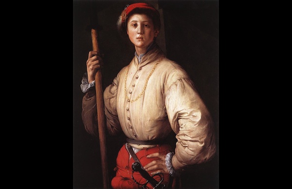
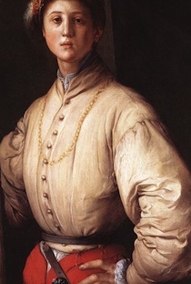
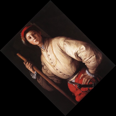
The information for an individual pixel can be extracted from an image in the same way an individual element of an array is referenced in Python. The next examples show how to extract the pixel at (120, 150) from the picture of the Portrait of a Halberdier painting, as demonstrated in Figure 4-2.

from SimpleCV import Image

img = Image('jacopo.png')

# Gets the information for the pixel located at
# x coordinate = 120, and y coordinate = 150
pixel = img[120, 150]

print pixel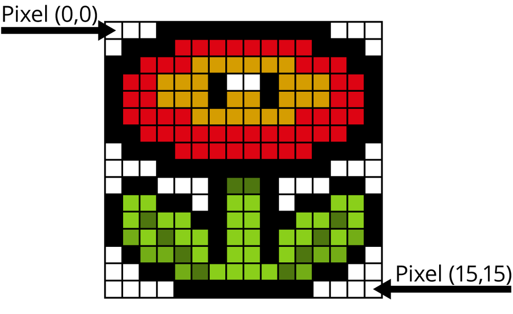

Figure 4-1. Pixels and coordinates. Note that (0, 0) is in the upper-left corner

Figure 4-2. Portrait of a Halberdier by Jacopo Pontormo

The value of pixel will become the RGB triplet for the pixel at (120, 150). As a result, print pixel returns (242.0, 222.0, 204.0).

The following example code does exactly the same thing, but uses the getPixel() function instead of the index of the array. This is the more object-oriented programming approach compared to extracting the pixel directly from the array.

from SimpleCV import Image

img = Image('jacopo.png')

# Uses getPixel() to get the information for the pixel located
# at x coordinate = 120, and y coordinate = 150
pixel = img.getPixel(120, 150)

print pixel

Tip

Want the grayscale value of a pixel in a color image? Rather than converting the whole image to grayscale, and then returning the pixel, use getGrayPixel(x, y).

Accessing pixels by their index can sometimes create problems. In the example above, trying to use img[1000, 1000] will throw an error, and img.getPixel(1000, 1000) will give a warning because the image is only 300×389. Because the pixel indexes start at zero, not one, the dimensions must be in the range 0-299 on the x-axis and 0-388 on the y-axis. To avoid problems like this, use the width and height properties of an image to find its dimensions. For example:

from SimpleCV import Image

img = Image('jacopo.png')

# Print the pixel height of the image
# Will print 300
print img.height

# Print the pixel width of the image
# Will print 389
print img.width

In addition to extracting RGB triplets from an image, it is also possible to change the image using an RGB triplet. The following example will extract a pixel from the image, zero out the green and blue components, preserving only the red value, and then put that back into the image.

from SimpleCV import Image

img = Image('jacopo.png')

# Retrieve the RGB triplet from (120, 150)
(red, green, blue) = img.getPixel(120, 150)  

# Change the color of the pixel+
img[120, 150] = (red, 0, 0)  

img.show()

By default, each pixel is returned as a tuple of the red, green, and blue components. (Chapter 5 covers this in more detail.) This conveniently stores each separate value in its own variable, appropriately named red, green, and blue.

Now instead of using the original value of green and blue, those are set to zero. Only the original red value is preserved. This effect is demonstrated in Figure 4-3:

Figure 4-3. On the left—the image with the new red pixel; on the right—a zoomed view of the changed pixel

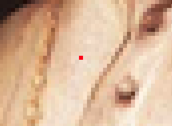
Since only one pixel was changed, it is hard to see the difference, but now the pixel at (120, 150) is a dark red color. To make it easier to see, resize the image to five times its previous size by using the resize() function.

from SimpleCV import Image

img = Image('jacopo.png')

# Get the pixel and change the color
(red, green, blue) = img.getPixel(120, 150)
img[120, 150] = (red, 0, 0)

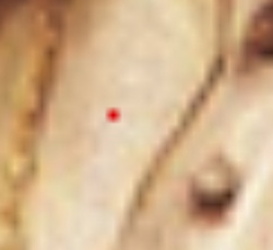
# Resize the image so it is 5 times bigger than its original size
bigImg = img.resize(img.width*5, img.height*5)

bigImg.show()

The much larger image should make it easier to see the red-only pixel that changed. Notice, however, that in the process of resizing the image, the single red pixel is interpolated, resulting in extra red in nearby pixels, as demonstrated in Figure 4-4.

Figure 4-4. The original red pixel after resizing

Right now, this looks like random fun with pixels with no actual purpose. However, pixel extraction is an important tool when trying to find and extract objects of a similar color. Most of these tricks are covered later in the book, but to provide a quick preview of how it is used, the following example looks at the color distance of other pixels compared with a given pixel, as shown in Figure 4-5.

from SimpleCV import Image
img = Image('jacopo.png')

# Get the color distance of all pixels compared to (120, 150)
distance = img.colorDistance(img.getPixel(120, 150))

# Show the resulting distances
distance.show()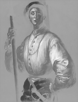

Figure 4-5. Color distance compared to the pixel at (100, 50)

Image Scaling

The block of code above shows the next major concept with images: scaling. In the above example, both the width and the height were changed by taking the img.height and img.width parameters and multiplying them by 5. In this next case, rather than entering the new dimensions, the scale() function will resize the image with just one parameter: the scaling factor. For example, the following code resizes the image to five times its original size.

from SimpleCV import Image

img = Image('jacopo.png')

# Scale the image by a factor of 5
bigImg = img.scale(5)

bigImg.show()

Caution

Notice that two different functions were used in the previous examples. The resize() function takes two arguments representing the new dimensions. The scale() function takes just one argument with the scaling factor (how many times bigger or smaller to make the image). When using the resize() function and the aspect ratio (the ratio of the width to height) changes, it can result in funny stretches to the picture, as is demonstrated in the next example.

from SimpleCV import Image

img = Image('jacopo.png')

# Resize the image, keeping the original height,
# but doubling the width
bigImg = img.resize(img.width * 2, img.height)

bigImg.show()

In this example, the image is stretched in the width dimension, but no change is made to the height, as demonstrated in Figure 4-6. To resolve this problem, use adaptive scaling with the adaptiveScale() function. It will create a new image with the dimensions requested. However, rather than wrecking the proportions of the original image, it will add padding. For example:

from SimpleCV import Image

# Load the image
img = Image('jacopo.png')

# Resize the image, but use the +adaptiveScale()+ function to maintain
# the proportions of the original image
adaptImg = img.adaptiveScale((img.width * 2, img.height))

adaptImg.show()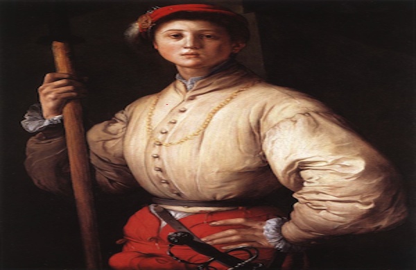

Figure 4-6. The poor Halberdier has gained weight

As you can see in Figure 4-7 in the resulting image, the original proportions are preserved, with the image content placed in the center of the image, and padding is added to the top and bottom of the image.

Figure 4-7. Resized with adaptive scaling

Note

The adaptiveScale() function takes a tuple of the image dimensions, not separate x and y arguments. Hence, the double parentheses.

Adaptive scaling is particularly useful when trying to enforce a standard image size on a collection of heterogeneous images. This example creates 50×50 thumbnail images in a directory called thumbnails.

from SimpleCV import ImageSet
from os import mkdir

# Create a local directory named thumbnails for storing the images
mkdir("thumbnails")

# Load the files in the current directory
set = ImageSet(".")

for img in set:
     print "Thumbnailing: " + img.filename

     # Scale the image to a +50 x 50+ version of itself,
     # and then save it in the thumbnails folder
     img.adaptiveScale((50, 50)).save("thumbnails/" + img.filename)

print "Done with thumbnails.  Showing slide show."

# Create an image set of all of the thumbnail images
thumbs = ImageSet("./thumbnails/")

# Display the set of thumbnailed images to the user
thumbs.show(3)

The adaptiveScale() function has an additional parameter, fit, that defaults to true. When fit is true, the function tries to scale the image as much as possible, while adding padding to ensure proportionality. When fit is false, instead of padding around the image to meet the new dimensions, it instead scales it in such a way that the smallest dimension of the image fits the desired size. Then it will crop the larger dimension so that the resulting image still fits the proportioned size.

A final variant of scaling is the embiggen() function (see Figure 4-8). This changes the size of the image by adding padding to the sides, but does not alter the original image. In some other image editing software, this is the equivalent of changing the canvas size without changing the image. The embiggen() function takes three arguments:

• A tuple with the width and height of the embiggened image.

• The color for the padding to place around the image. By default, this is black.

• A tuple of the position of the original image on the larger canvas. By default, the image is centered.

from SimpleCV import Image, Color

img = Image('jacopo.png')

# Embiggen the image, put it on a green background, in the upper right
emb = img.embiggen((350, 400), Color.GREEN, (0, 0))

emb.show()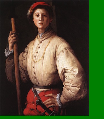

Figure 4-8. An embiggened image with changed color and position

Warning

The embiggen() function will throw a warning if trying to embiggen an image into a smaller set of dimensions. For example, the 300x389 example image cannot be embiggened into a 150×200 image.

Image Cropping

In many image processing applications, only a portion of the image is actually important. For instance, in a security camera application, it may be that only the door—and whether anyone is coming or going—is of interest. Cropping speeds up a program by limiting the processing to a “region of interest” rather than the entire image. The SimpleCV framework has two mechanisms for cropping: the crop() function and Python’s slice notation.

Image.crop() takes four arguments that represent the region to be cropped. The first two are the x and y coordinates for the upper left corner of the region to be cropped, and the last two are the width and height of the area to be cropped.

For example, to crop out just the bust in the picture, you could use the following code. The resulting image is shown in Figure 4-9:

from SimpleCV import Image

img = Image('jacopo.png')

# Crop starting at +(50, 5)+ for an area 200 pixels wide by 200 pixels tall
cropImg = img.crop(50, 5, 200, 200)

cropImg.show()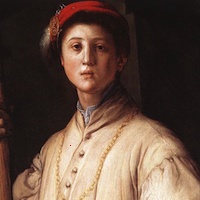

Figure 4-9. Cropping to just the bust in the image

When performing a crop, it is sometimes more convenient to specify the center of the region of interest rather than the upper left corner. To crop an image from the center, add one more parameter, centered = True, with the result shown in Figure 4-10.

from SimpleCV import Image

img = Image('jacopo.png')

# Crop the image starting at the center of the image
cropImg = img.crop(img.width/2, img.height/2, 200, 200, centered=True)

cropImg.show()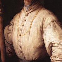

Figure 4-10. The image cropped around the center

Crop regions can also be defined by image features. Many of these features are covered later in the book, but blobs were briefly introduced in previous chapters. As with other features, the SimpleCV framework can crop around a blob. For example, a blob detection can also find the torso in the picture.

from SimpleCV import Image

img = Image('jacopo.png')

blobs = img.findBlobs()  

img.crop(blobs[-1]).show()  

This will find the blobs in image.

The findBlobs() function returns the blobs in ascending order by size. This will be covered in greater detail in later chapters. In this example, that means the bust is the largest blob.

Once cropped, the image should look like Figure 4-11.

Figure 4-11. The cropped painting using blobs

The crop function is also implemented for Blob features, so the above code could also be written as follows. Notice that the crop() function is being called directly on the blob object instead of the image object.

from SimpleCV import Image

img = Image('jacopo.png')

blobs = img.findBlobs()

# Crop function being called directly on the blob object
blobs[-1].crop().show()

Image Slicing

For the Python aficionados, it is also possible to do cropping by directly manipulating the two dimensional array of the image. Individual pixels could be extracted by treating the image like an array and specifying the (x, y) coordinates. Python can also extract ranges of pixels as well. For example, img[start_x:end_x, start_y:end_y] provides a cropped image from (start_x, start_y) to (end_x, end_y). Not including a value for one or more of the coordinates means that the border of the image will be used as the start or end point. So something like img[ : , 300:] works. That will select all of the x values and all of the y values that are greater than 300. In essence, any of Python’s functions for extracting subsets of arrays will also work to extract parts of an image, and thereby return a new image. Because of this, images can be cropped using Python’s slice notation instead of the crop function:

from SimpleCV import Image

img = Image('jacopo.png')

# Cropped image that is 200 pixels wide and 200 pixels tall starting at (50, 5).
cropImg = img[50:250,5:205]

cropImg.show()

Note

When using slice notation, specify the start and end locations. When using crop, specify a starting coordinate and a width and height.

Transforming Perspectives: Rotate, Warp, and Shear

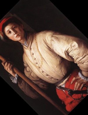
When writing a vision application, is is common to assume that the camera is positioned squarely to view an image and that the top of the image is “up.” However, sometimes the camera is held at an angle to an object or not oriented squarely to the image. This can complicate the image analysis. Fortunately, sometimes this can be fixed with rotations, shears, and skews.

Spin, Spin, Spin Around

The simplest operation is to rotate the image so that it is correctly oriented. This is accomplished with the rotate() function, which only has one required argument, angle. This value is the angle, in degrees, to rotate the image. Negative values for the angle rotate the image clockwise and positive values rotate it counterclockwise. To rotate the image 45 degrees counterclockwise:

from SimpleCV import Image

img = Image('jacopo.png')

# Rotate the image counter-clockwise 45 degrees
rot = img.rotate(45)

rot.show()

The resulting rotated image is shown in Figure 4-12.

Figure 4-12. The image rotated 45 degrees to the left

Generally, rotation means to rotate around the center point. However, a different axis of rotation can be chosen by passing an argument to the point parameter. This parameter is a tuple of the (x, y) coordinate for the new point of rotation.

from SimpleCV import Image

img = Image('jacopo.png')

# Rotate the image around the coordinates +(16, 16)+
rot = img.rotate(45, point=(16, 16))

rot.show()

The rotated image is shown in Figure 4-13. Notice that the image was cropped during the rotation.

Figure 4-13. Rotation around (16, 16)

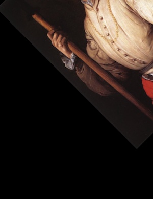
Note that when the image is rotated, if part of the image falls outside the original image dimensions, that section is cropped. The rotate() function has a parameter called fixed to control this. When fixed is set to false, the algorithm will return a resized image, where the size of the image is set to include the whole image after rotation.

For example, to rotate the image without clipping off the corners:

from SimpleCV import Image

img = Image('jacopo.png')

# Rotate the image and then resize it so the content isn't cropped
rot = img.rotate(45, fixed=False)

rot.show()

The image of the dizzy halberdier is shown in Figure 4-14.

Figure 4-14. Rotation with the canvas resized to fit the whole image

Note

Even when defining a rotation point, if the fixed parameter is false, the image will still be rotated about the center. The additional padding around the image essentially compensates for the alternative rotation point.

Finally, for convenience, the image can be scaled at the same time that it is rotated. This is done with the scale parameter. The value of the parameter is a scaling factor, similar to the scale function.

from SimpleCV import Image

img = Image('jacopo.png')

# Rotate the image and make it half the size
rot = img.rotate(90, scale=.5)

rot.show()

Flipping Images

Similar to rotating, an image can also be flipped across its horizontal or vertical axis (Figure 4-15). This is done with the flipHorizontal() and flipVertical() functions. To flip the image across its horizontal axis:

from SimpleCV import Image

img = Image('jacopo.png')

# Flip the image along the horizontal axis and then display the results
flip = img.flipHorizontal()

flip.show()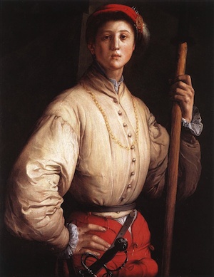

Figure 4-15. A mirror image of the Jacopo Pontormo painting

The following example applies the horizontal flip to make a webcam act like a mirror, perhaps so you can check your hair or apply your makeup with the aid of your laptop.

from SimpleCV import Camera, Display

cam = Camera()

# The image captured is just used to match Display size with the Camera size
disp = Display( (cam.getProperty('width'), cam.getProperty('height')) )

while disp.isNotDone():
     cam.getImage().flipHorizontal().save(disp)

Note that a flip is not the same as a rotation by 180 degrees. Figure 4-16 demonstrates the difference between flips and rotations.

Figure 4-16. Left: The original image; Center: The image rotated 180 degrees; Right: The image flipped vertically

Shears and Warps

Images or portions of an image are sometimes skewed to make them fit into another shape. A common example of this is overlaying an image on top of a square object that is viewed at an angle. When viewing a square object at an angle, the corners of the square no longer appear to be 90 degrees. Instead, to align a square object to fit into this angular space, its edges must be adjusted. Underneath the hood, it is performing an affine transformation, though this is more commonly called a shear.

Tip

The tricky part when doing warps is finding all the (x, y) coordinates. Use Camera.live() and click on the image to help find the coordinates for the skew.

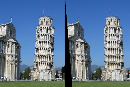
To demonstrate shearing, the following block of code can be used to fix the Leaning Tower of Pisa (see Figure 4-17). Granted, it makes the other building in the picture tip too far to the left, but some people are never happy.

from SimpleCV import Image

img = Image('pisa.png')

corners = [(0, 0), (450, 0), (500, 600), (50, 600)]  

straight = img.shear(corners)  

straight.show()

This is a list of the corner points for the sheared image. The original image is 450 x 600 pixels. To fix the tower, the lower right corners are shifted by 50 pixels to the right. Note that the points for the new shape are passed in clockwise order, starting from the top left corner.

Next simply call the shear() function, passing the list of new corner points for the image.

Figure 4-17. Left: The original leaning tower; Right: The repaired version of the tower

In addition to shearing, images can also be warped by using the warp() function. Warping also takes an array of corner points as its parameters. Similar to shearing, it is used to stretch an image and fit it into a nonrectangular space.

Note

A shear will maintain the proportions of the image. As such, sometimes the actual corner points will be adjusted by the algorithm. In contrast, a warp can stretch the image so that it fits into any new shape.

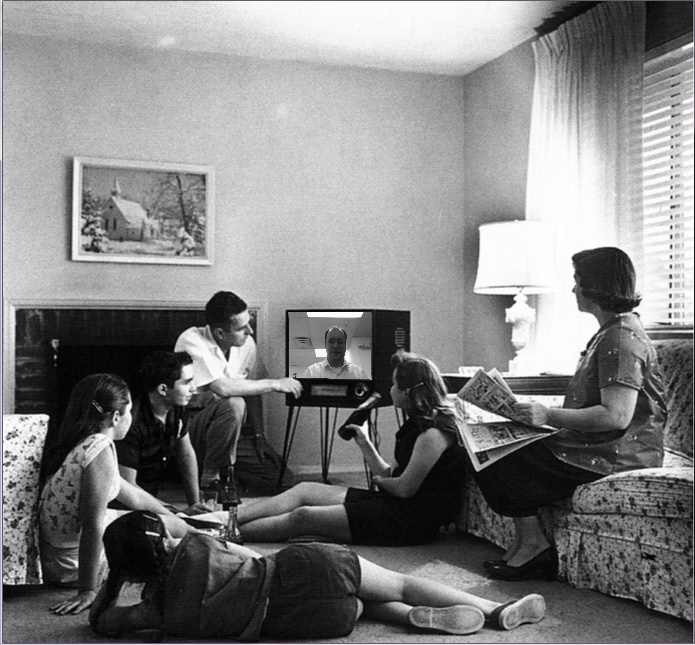
Everybody wants to be on television, but with this next example, now anyone can have the chance to be on TV and go back in time. The impudent might even call it a “time warp”…

from SimpleCV import Camera, Image, Display

tv_original = Image("family.png")  

tv_coordinates = [(285,  311), (367, 311), (368, 378), (286, 376)]  

tv_mask = Image(tv_original.size()).invert().warp(tv_coordinates)  

tv = tv_original - tv_mask  

cam = Camera()

disp = Display(tv.size())

# While the window is open, keep updating updating
# the TV with images from the camera
while disp.isNotDone():

     bwimage = cam.getImage().grayscale().resize(tv.width, tv.height)  

     on_tv = tv + bwimage.warp(tv_coordinates)  

     on_tv.save(disp)

This is the image we’ll be using for the background. The image captured via the webcam will be placed on top of the TV.

These are the coordinates of the corners of the television.

Image(tv_original.size()) creates a new image that has the same size as the original TV image. By default, this is an all black image. The invert function makes it white. The warp function then creates a white warped region in the middle, based on the coordinates previously defined for the TV. The result is Figure 4-18.

Using image subtraction, the TV is now removed from the image. This is a trick that will be covered more extensively in the next chapter.

Now capture an image from the camera. To be consistent with the black and white background image, convert it to grayscale. In addition, since this image will be added to the background image, it needs to be resized to match the background image.

Finally, do another warp to make the image from the camera fit into the TV region of the image. This is then added onto the background image (Figure 4-19).

Figure 4-18. The mask for the TV image, which is white where the TV sits and black otherwise

Figure 4-19. Sample output from this example, with our handsome book author appearing on the television

Image Morphology

It is always preferable to control the real-world lighting and environment in order to maximize the quality of an image. However, even in the best of circumstances, an image will include pixel-level noise. That noise can complicate the detection of features on the image, so it is important to clean it up. This is the job of morphology.

Binarization

Many morphology functions work with color images, but they are easiest to see in action when working with a binary (2-color) image. Binary literally means the image is black and white, with no shades of gray. To create a binary image, use the binarize() function:

from SimpleCV import Image

img = Image('jacopo.png')

imgBin = img.binarize()

imgBin.show()

The output is demonstrated in Figure 4-20. Notice that it is purely black and white (no gray).

Figure 4-20. The Jacopo painting, binarized

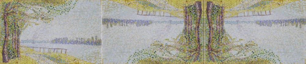
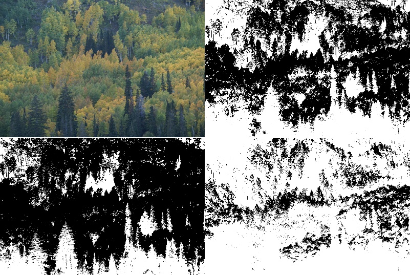
Whenever an image is binarized, the system needs to know which pixels get converted to black, and which to white. This is called a “threshold”, and any pixel where the grayscale value falls under the threshold is changed to white. Any pixel above the threshold is changed to black. By default, the SimpleCV framework uses a technique called Otsu’s method to dynamically determine the binarized values. However, the binarize function also takes a parameter value between 0-255. The following example code shows the use of binarization at several levels:

from SimpleCV import Image

img = Image('trees.png')

# Using Otsu's method
otsu = img.binarize()

# Specify a low value
low = img.binarize(75)

# Specify a high value
high = img.binarize(125)

img = img.resize(img.width*.5, img.height*.5)
otsu = otsu.resize(otsu.width*.5, otsu.height*.5)
low = low.resize(low.width*.5, low.height*.5)
high = high.resize(high.width*.5, high.height*.5)


top  = img.sideBySide(otsu)
bottom = low.sideBySide(high)
combined = top.sideBySide(bottom, side="bottom")

combined.show()

Figure 4-21 demonstrates the output of these four different thresholds.

Figure 4-21. Top Left: The original imag;e Top Right: Binarized with Otsu’s method; Bottom Left: Low threshold value; Bottom Right: High threshold value

Dilation and Erosion

Once the image is converted into a binary format, there are four common morphological operations: dilation, erosion, opening, and closing. Dilation and erosion are conceptually similar. With dilation, any background pixels (black) that are touching an object pixel (white) are turned into a white object pixel. This has the effect of making objects bigger, and merging adjacent objects together. Erosion does the opposite. Any foreground pixels (white) that are touching a background pixel (black) are converted into a black background pixel. This makes the object smaller, potentially breaking large objects into smaller ones.

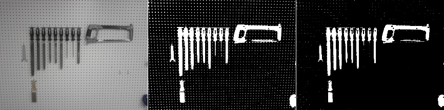
For the examples in this section, consider the case of a pegboard with tools. The small holes in pegboard can confuse feature detection algorithms. Tricks like morphology can help clean up the image. The first example shows dilating the image. In particular, notice that after binarizing, some of the parts of the tools have disappeared where there was glare. To try to get these back, use dilation to fill in some of the missing parts.

from SimpleCV import Image

img = Image('pegboard.png')

# Binarize the image so that it's a black and white image
imgBin = img.binarize()

# Show the effects of dilate() on the image
imgBin.dilate().show()

Notice in Figure 4-22 that although this filled in some of the gaps in the tools, the pegboard holes grew. This is the opposite of the desired effect. To get rid of the holes, use the erode() function.

Figure 4-22. Left: The original image Center: Binarized image Right: Dilated image

from SimpleCV import Image

img = Image('pegboard.png')

imgBin = img.binarize()

# Like the previous example, but erode()
imgBin.erode().show()

As you can see in Figure 4-23, this essentially has the opposite effect. It made a few of the gaps in the image worse, such as with the saw blade. On the other hand, it eliminated most of the holes on the peg board.

Figure 4-23. Left: The original image; Center: Binarized image; Right: Eroded image

While the dilate() function helps fill in the gaps, it also amplifies some of the noise. In contrast, the erode() function eliminates a bunch of noise, but at the cost of some good data. The solution is to combine these functions together. In fact, the combinations are so common, they have their own named functions: morphOpen() and morphClose(). The morphOpen() function erodes and then dilates the image. The erosion step eliminates very small (noise) objects, following by a dilation which more or less restores the original size objects to where they were before the erosion. This has the effect of removing specks from the image. In contrast, morphClose() first dilates and then erodes the image. The dilation first fills in small gaps between objects. If those gaps were small enough, the dilation completely fills them in, so that the subsequent erosion does not reopen the hole. This has the effect of filling in small holes. In both cases, the goal is to reduce the amount of noise in the image.

For example, consider the use of morphOpen() on the pegboard. This eliminates a lot of the pegboard holes while still trying to restore some of the damage to the tools created by the erosion, as demonstrated in Figure 4-24.

from SimpleCV import Image

img = Image('pegboard.png')

imgBin = img.binarize()

# +morphOpen()+ erodes and then dilates the image
imgBin.morphOpen().show()

Figure 4-24. Left: The original image; Center: Binarized image; Right: Image after morphOpen()

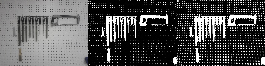
Although this helped a lot, it still leaves a lot of the pegs in the pegboard. Sometimes, the trick is simply to do multiple erosions followed by multiple dilations. To simplify this process, the dilate() and erode() functions each take a parameter representing the number of times to repeat the function. For instance, dilate(5) performs a dilation five times, as demonstrated in Figure 4-25.

from SimpleCV import Image

img = Image('pegboard.png')

# Dilate the image twice to fill in gaps
noPegs = img.dilate(2)

# Then erode the image twice to remove some noise
filled = noPegs.erode(2)

allThree = img.sideBySide(noPegs.sideBySide(filled))
allThree.scale(.5).show()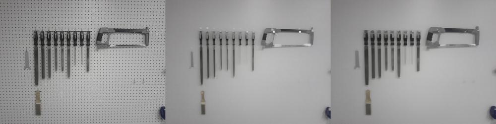

Figure 4-25. Left: The original image; Center: Dilated image; Right: Eroded after dilation

Examples

The examples in this section demonstrate both a fun application and a practical application. On the fun side, it shows how to do a spinning effect with the camera, using the rotate() function. On the practical side, it shows how to shear an object viewed at an angle, and then use the corrected image to perform a basic measurement.

The SpinCam

This is a very simple script which continually rotates the output of the camera. It continuously captures images from the camera. It also progressively increments the angle of rotation, making it appear as though the video feed is spinning.

from SimpleCV import Camera

cam = Camera()
display = Display()

# This variable saves the last rotation, and is used
# in the while loop to increment the rotation
rotate = 0

while display.isNotDone():
     rotate = rotate + 5  
     cam.getImage().rotate(rotate).save(display)  

Increment the amount of rotation by five degrees. Note that when the rotation exceeds 360 degrees, it automatically loops back around.

Take a new image and rotate by the amount computed in the previous step. Then display the image.

Warp and Measurement

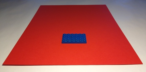
The second example is slightly more practical. Measuring objects is covered in more detail later in this book, but this example provides a general introduction. The basic idea is to compare the object being measured to an object of a known size. For example, if an object is sitting on top of an 8.5×11 inch piece of paper, the relative size of the objects can be used to compute the size. However, this is complicated if the paper is not square to the camera. This example shows how to fix that with the warp() function. The image in Figure 4-26 is used to measure the size of the small building block on the piece of paper.

Figure 4-26. The original image of the building block on paper

from SimpleCV import Image

img = Image('skew.png')

# Warp the picture to straighten the paper
corners = [(0, 0), (480, 0), (336, 237), (147, 237)]  

warped = img.warp(corners)  

# Find the blob that represents the paper
bgcolor = warped.getPixel(240, 115)

dist = warped.colorDistance(bgcolor)  

blobs = dist.invert().findBlobs()  

paper = blobs[-1].crop()  

# Find the blob that represents the toy
toyBlobs = paper.invert().findBlobs()

toy = toyBlobs[-1].crop()  

# Use the toy block/paper ratio to compute the size
paperSize = paper.width
toySize = toy.width

print float(toySize) / float(paperSize) * 8.5  

These are the coordinates for the four corners of the paper. A good way to help identify the corner points is to use the SimpleCV shell to load the image, and then use the image.live() function to display it. Then left-click on the displayed image to find the coordinates of the paper corners.

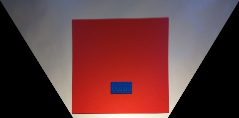
This warps the image to square the edges of the piece of paper, as shown in Figure 4-27.

Use the image.live() trick to also find the color of the paper. This makes it easier to find the part of the image that is the paper versus other background objects. The image below shows the result. Notice that the paper is black whereas the rest of the image is represented in various shades of gray.

By making the paper black, it is easier to pull it out of the image with the findBlobs() function.

Next, crop the original image down to just the largest blob (the paper), as represented by blobs[-1]. This creates a new image that is just the paper.

Now looking at just the area of the paper, use the findBlobs function again to locate the toy block. Create an image of the block by cropping it from off the paper.

Using the ratio of the width of the paper and the toy block, combined with the fact that the paper is 8.5 inches wide, compute the size of the block, which is 1.87435897436, which matches the objects size of 1.875 inches.

Note that this example works best when measuring relatively flat objects. When adjusting the skew, it makes the top of the object appear larger than the bottom, which can result in an over-reported size. Later chapters will discuss blobs in greater depth, including working with blob properties to get a more accurate measurement.

See Figure 4-28 for another example of color distance.

Figure 4-27. The image warped to square the sides of the paper

Figure 4-28. Color distance from the red background, making it easier to extract the paper and the block