Machine learning exists at the intersection of traditional mathematics and statistics with software engineering and computer science. In this book, we will describe several tools from traditional statistics that allow you to make sense of the world. Statistics has almost always been concerned with learning something interpretable from data, whereas machine learning has been concerned with turning data into something practical and usable. This contrast makes it easier to understand the term machine learning: Machine learning is concerned with teaching computers something about the world, so that they can use that knowledge to perform other tasks. In contrast, statistics is more concerned with developing tools for teaching humans something about the world, so that they can think more clearly about the world in order to make better decisions.
In machine learning, the learning occurs by extracting as much information from the data as possible (or reasonable) through algorithms that parse the basic structure of the data and distinguish the signal from the noise. After they have found the signal, or pattern, the algorithms simply decide that everything else that’s left over is noise. For that reason, machine learning techniques are also referred to as pattern recognition algorithms. We can “train” our machines to learn about how data is generated in a given context, which allows us to use these algorithms to automate many useful tasks. This is where the term training set comes from, referring to the set of data used to build a machine learning process. The notion of observing data, learning from it, and then automating some process of recognition is at the heart of machine learning and forms the primary arc of this book. Two particularly important types of patterns constitute the core problems we’ll provide you with tools to solve: the problem of classification and the problem of regression, which will be introduced over the course of this book.
In this book, we assume a relatively high degree of knowledge in basic programming techniques and algorithmic paradigms. That said, R remains a relatively niche language, even among experienced programmers. In an effort to establish the same starting point for everyone, this chapter provides some basic information on how to get started using the R language. Later in the chapter we will provide an extended case study for working with data in R.
Warning
This chapter does not provide a complete introduction to the R programming language. As you might expect, no such introduction could fit into a single book chapter. Instead, this chapter is meant to prepare the reader for the tasks associated with doing machine learning in R, specifically the process of loading, exploring, cleaning, and analyzing data. There are many excellent resources on R that discuss language fundamentals such as data types, arithmetic concepts, and coding best practices. In so far as those topics are relevant to the case studies presented here, we will touch on all of these issues; however, there will be no explicit discussion of these topics. For those interested in reviewing these topics, many of these resources are listed in Table 1-3.
If you have never seen the R language and its syntax before, we highly recommend going through this introduction to get some exposure. Unlike other high-level scripting languages, such as Python or Ruby, R has a unique and somewhat prickly syntax and tends to have a steeper learning curve than other languages. If you have used R before but not in the context of machine learning, there is still value in taking the time to go through this review before moving on to the case studies.
R is a language and environment for statistical computing and graphics....R provides a wide variety of statistical (linear and nonlinear modeling, classical statistical tests, time-series analysis, classification, clustering, ...) and graphical techniques, and is highly extensible. The S language is often the vehicle of choice for research in statistical methodology, and R provides an Open Source route to participation in that activity.
—The R Project for Statistical Computing, http://www.r-project.org/
The best thing about R is that it was developed by statisticians. The worst thing about R is that...it was developed by statisticians.
R is an extremely powerful language for manipulating and analyzing data. Its meteoric rise in popularity within the data science and machine learning communities has made it the de facto lingua franca for analytics. R’s success in the data analysis community stems from two factors described in the preceding epitaphs: R provides most of the technical power that statisticians require built into the default language, and R has been supported by a community of statisticians who are also open source devotees.
There are many technical advantages afforded by a language
designed specifically for statistical computing. As the description from
the R Project notes, the language provides an open source bridge to S,
which contains many highly specialized statistical operations as base
functions. For example, to perform a basic linear regression in R, one
must simply pass the data to the lm
function, which then returns an object containing detailed information
about the regression (coefficients, standard errors, residual values,
etc.). This data can then be visualized by passing the results to the
plot function, which is designed to
visualize the results of this analysis.
In other languages with large scientific computing communities,
such as Python, duplicating the functionality of lm requires the use of several third-party
libraries to represent the data (NumPy), perform the analysis (SciPy),
and visualize the results (matplotlib). As we will see in the following
chapters, such sophisticated analyses can be performed with a single
line of code in R.
In addition, as in other scientific computing environments, the fundamental data type in R is a vector. Vectors can be aggregated and organized in various ways, but at the core, all data is represented this way. This relatively rigid perspective on data structures can be limiting, but is also logical given the application of the language. The most frequently used data structure in R is the data frame, which can be thought of as a matrix with attributes, an internally defined “spreadsheet” structure, or relational database-like structure in the core of the language. Fundamentally, a data frame is simply a column-wise aggregation of vectors that R affords specific functionality to, which makes it ideal for working with any manner of data.
Warning
For all of its power, R also has its disadvantages. R does not scale well with large data, and although there have been many efforts to address this problem, it remains a serious issue. For the purposes of the case studies we will review, however, this will not be an issue. The data sets we will use are relatively small, and all of the systems we will build are prototypes or proof-of-concept models. This distinction is important because if your intention is to build enterprise-level machine learning systems at the Google or Facebook scale, then R is not the right solution. In fact, companies like Google and Facebook often use R as their “data sandbox” to play with data and experiment with new machine learning methods. If one of those experiments bears fruit, then the engineers will attempt to replicate the functionality designed in R in a more appropriate language, such as C.
This ethos of experimentation has also engendered a great sense of community around the language. The social advantages of R hinge on this large and growing community of experts using and contributing to the language. As Bo Cowgill alludes to, R was borne out of statisticians’ desire to have a computing environment that met their specific needs. Many R users, therefore, are experts in their various fields. This includes an extremely diverse set of disciplines, including mathematics, statistics, biology, chemistry, physics, psychology, economics, and political science, to name a few. This community of experts has built a massive collection of packages on top of the extensive base functions in R. At the time of writing, CRAN, the R repository for packages, contained over 2,800 packages. In the case studies that follow, we will use many of the most popular packages, but this will only scratch the surface of what is possible with R.
Finally, although the latter portion of Cowgill’s statement may
seem a bit menacing, it further highlights the strength of the R
community. As we will see, the R language has a particularly odd syntax
that is rife with coding “gotchas” that can drive away even experienced
developers. But all grammatical grievances with a language can
eventually be overcome, especially for persistent hackers. What is more
difficult for nonstatisticians is the liberal assumption of familiarity
with statistical and mathematical methods built into R functions. Using
the lm function as an example, if you
had never performed a linear regression, you would not know to look for
coefficients, standard errors, or residual values in the results. Nor
would you know how to interpret those results.
But because the language is open source, you are always able to look at the code of a function to see exactly what it is doing. Part of what we will attempt to accomplish with this book is to explore many of these functions in the context of machine learning, but that exploration will ultimately address only a tiny subset of what you can do in R. Fortunately, the R community is full of people willing to help you understand not only the language, but also the methods implemented in it. Table 1-1 lists some of the best places to start.
Table 1-1. Community resources for R help
| Resource | Location | Description |
|---|---|---|
| RSeek | http://rseek.org/ | When the core development team decided to create an open source version of S and call it R, they had not considered how hard it would be to search for documents related to a single-letter language on the Web. This specialized search tool attempts to alleviate this problem by providing a focused portal to R documentation and information. |
| Official R mailing lists | http://www.r-project.org/mail.html | There are several mailing lists dedicated to the R language, including announcements, packages, development, and—of course—help. Many of the language’s core developers frequent these lists, and responses are often quick and terse. |
| StackOverflow | http://stackoverflow.com/questions/tagged/r | Hackers will know StackOverflow.com as one of the premier web resources for coding tips in any language, and the R tag is no exception. Thanks to the efforts of several prominent R community members, there is an active and vibrant collection of experts adding and answering R questions on StackOverflow. |
| #rstats Twitter hash-tag | http://search.twitter.com/search?q=%23rstats | There is also a very active community of R users on Twitter, and they have designated the #rstats hash tag as their signifier. The thread is a great place to find links to useful resources, find experts in the language, and post questions—as long as they can fit into 140 characters! |
| R-Bloggers | http://www.r-bloggers.com/ | There are hundreds of people blogging about how they use R in their research, work, or just for fun. R-bloggers.com aggregates these blogs and provides a single source for all things related to R in the blogosphere, and it is a great place to learn by example. |
| Video Rchive | http://www.vcasmo.com/user/drewconway | As the R community grows, so too do the number of regional meetups and gatherings related to the language. The Rchive attempts to document the presentations and tutorials given at these meetings by posting videos and slides, and now contains presentations from community members all over the world. |
The remainder of this chapter focuses on getting you set up with R and using it. This includes downloading and installing R, as well as installing R packages. We conclude with a miniature case study that will serve as an introduction to some of the R idioms we’ll use in later chapters. This includes issues of loading, cleaning, organizing, and analyzing data.
Like many open source projects, R is distributed by a series of regional mirrors. If you do not have R already installed on your machine, the first step is to download it. Go to http://cran.r-project.org/mirrors.html and select the CRAN mirror closest to you. Once you have selected a mirror, you will need to download the appropriate distribution of R for whichever operating system you are running.
R relies on several legacy libraries compiled from C and Fortran. As such, depending on your operating system and your familiarity with installing software from source code, you may choose to install R from either a compiled binary distribution or the source. Next, we present instructions for installing R on Windows, Mac OS X, and Linux distributions, with notes on installing from either source or binaries when available.
Finally, R is available in both 32- and 64-bit versions. Depending on your hardware and operating system combination, you should install the appropriate version.
For Windows operating systems, there are two subdirectories available to install R: base and contrib. The latter is a directory of compiled Windows binary versions of all of the contributed R packages in CRAN, whereas the former is the basic installation. Select the base installation, and download the latest compiled binary. Installing contributed packages is easy to do from R itself and is not language-specific; therefore, it is not necessary to to install anything from the contrib directory. Follow the on-screen instructions for the installation.
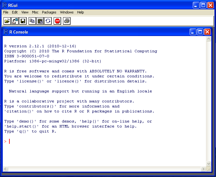
Once the installation has successfully completed, you will have an R application in your Start menu, which will open the RGui and R Console, as pictured in Figure 1-1.
For most standard Windows installations, this process should proceed without any issues. If you have a customized installation or encounter errors during the installation, consult the R for Windows FAQ at your mirror of choice.
Fortunately for Mac OS X users, R comes preinstalled with the
operating system. You can check this by opening
Terminal.app and simply typing
R at the command line. You are now ready to
begin! For some users, however, it will be useful to have a GUI
application to interact with the R Console. For this you will need
to install separate software. With Mac OS X, you have the option of
installing from either a compiled binary or the source. To install
from a binary—recommended for users with no experience using a Linux
command line—simply download the latest version at your mirror of
choice at http://cran.r-project.org/mirrors.html, and follow
the on-screen instructions. Once the installation is complete, you
will have both R.app (32-bit) and
R64.app (64-bit) available in your
Applications folder. Depending on your version
of Mac OS X and your machine’s hardware, you may choose which
version you wish to work with.
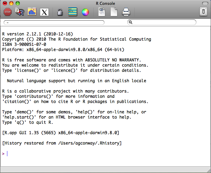
As with the Windows installation, if you are installing from a binary, this process should proceed without any problems. When you open your new R application, you will see a console similar to the one pictured in Figure 1-2.
Note
If you have a custom installation of Mac OS X or wish to customize the installation of R for your particular configuration, we recommend that you install from the source code. Installing R from source on Mac OS X requires both the C and Fortran compilers, which are not included in the standard installation of the operating system. You can install these compilers using the Mac OS X Developers Tools DVD included with your original Mac OS X installation package, or you can install the necessary compilers from the tools directory at the mirror of your choice.
Once you have all of the necessary compilers to install from source, the process is the typical configure, make, and install procedure used to install most software at the command line. Using Terminal.app, navigate to the folder with the source code and execute the following commands:
$ ./configure
$ make
$ make install
Depending on your permission settings, you may have to invoke
the sudo command as a prefix to
the configuration step and provide your system password. If you
encounter any errors during the installation, using either the
compiled binary distribution or the source code, consult the
R for Mac OS X FAQ at the mirror
of your choice.
As with Mac OS X, R comes preinstalled on many Linux
distributions. Simply type R at
the command line, and the R console will be loaded. You can now
begin programming! The CRAN mirror also includes installations
specific to several Linux distributions, with instructions for
installing R on Debian, RedHat, SUSE, and Ubuntu. If you use one of
these installations, we recommend that you consult the instructions
for your operating system because there is considerable variance in
the best practices among Linux distributions.
R is a scripting language, and therefore the majority of the work done in the case studies that follow will be done within an IDE or text editor, rather than directly inputted into the R console. As we show in the next section, some tasks are well suited for the console, such as package installation, but primarily you will want to work within the IDE or text editor of your choice.
For those running the GUI in either Windows or Mac OS X, there is a basic text editor available from that application. By either navigating to File→New Document from the menu bar or clicking on the blank document icon in the header of the window (highlighted in Figure 1-3), you will open a blank document in the text editor. As a hacker, you likely already have an IDE or text editor of choice, and we recommend that you use whichever environment you are most comfortable in for the case studies. There are simply too many options to enumerate here, and we have no intention of inserting ourselves in the infamous Emacs versus Vim debate.

There are many well-designed, -maintained, and -supported R packages related to machine learning. With respect to the case studies we will describe, there are packages for dealing with spatial data, text analysis, network structures, and interacting with web-based APIs, among many others. As such, we will be relying heavily on the functionality built into several of these packages.
Loading packages in R is very straightforward. There are two
functions to perform this: library
and require. There are some subtle
differences between the two, but for the purposes of this book, the
primary difference is that require
will return a Boolean (TRUE or
FALSE) value, indicating whether
the package is installed on the machine after attempting to load it.
For example, in Chapter 6 we
will use the tm package to tokenize text. To load
these packages, we can use either the library or require functions. In the following example,
we use library to load tm but use require for XML.
By using the print
function, we can see that we have XML installed
because a Boolean value of TRUE was
returned after the package was loaded:
library(tm)
print(require(XML))
#[1] TRUE
If we did not have XML
installed—i.e., if require returned FALSE—then we would need to install that
package before proceeding.
Note
If you are working with a fresh installation of R, then you will have to install a number of packages to complete all of the case studies in this book.
There are two ways to install packages in R: either with the
GUI or with the install.packages
function from the console. Given the intended audience for this book,
we will be interacting with R exclusively from the console during the
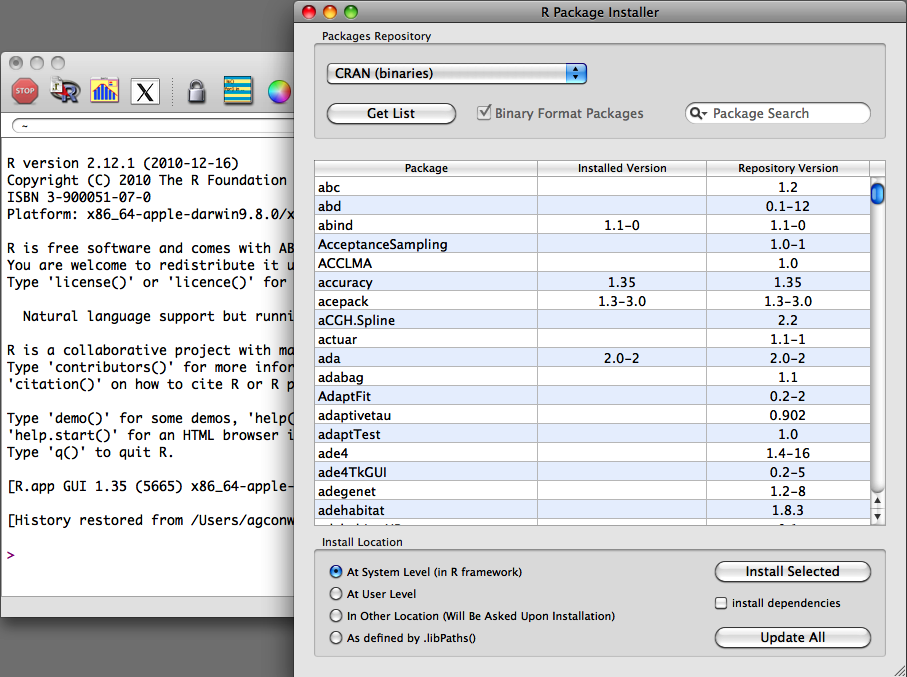
case studies, but it is worth pointing out how to use the GUI to
install packages. From the menu bar in the application, navigate to
Packages & Data→Package Installer,
and a window will appear, as displayed in Figure 1-4. From the
Package Repository drop-down, select either “CRAN (binaries)”or “CRAN
(sources)”, and click the Get List button to load all of the packages
available for installation. The most recent version of packages will
be available in the “CRAN (sources)” repository, and if you have the
necessary compilers installed on your machine, we recommend using this
sources repository. You can now select the package you wish to install
and click Install Selected to install the packages.
The install.packages function
is the preferred way to install packages because it provides greater
flexibility in how and where packages get installed. One of the
primary advantages of using install.packages is that it allows you to
install from local source code as well as from CRAN. Though uncommon,
occasionally you may want to install a package that is not yet
available on CRAN—for example, if you’re updating to an experimental
version of a package. In these cases you will need to install from
source:
install.packages("tm", dependencies=TRUE)
setwd("~/Downloads/")
install.packages("RCurl_1.5-0.tar.gz", repos=NULL, type="source")
In the first example, we use the default settings to
install the tm package from CRAN.
The tm provides a function used to
do text mining, and we will use it in Chapter 3 to perform classifications
on email text. One useful parameter in the install.packages function is suggests, which by default is set to
FALSE, but if activated will
instruct the function to download and install any secondary packages
used by the primary installation. As a best practice, we recommend
always setting this to TRUE,
especially if you are working with a clean installation of R.
Alternatively, we can also install directly from compressed
source files. In the previous example, we installed the RCurl package from the source code available
on the author’s website. Using the setwd function
to make sure the R working directory is set to the directory where the
source file has been saved, we can simply execute the command shown
earlier to install directly from the source code. Note the two
parameters that have been altered in this case. First, we must tell
the function not to use one of the CRAN repositories by setting
repos=NULL, and we also specify the
type of installation using type="source".
Table 1-2. R packages used in Machine Learning for Hackers
| Name | Location | Author(s) | Description and use |
|---|---|---|---|
arm | http://cran.r-project.org/web/packages/arm/ | Andrew Gelman, et al. | Package for doing multilevel/hierarchical regression models. |
ggplot2 | http://cran.r-project.org/web/packages/glmnet/index.html | Hadley Wickham | An implementation of the grammar of graphics in R. The premier package for creating high-quality graphics. |
glmnet | http://had.co.nz/ggplot2/ | Jerome Friedman, Trevor Hastie, and Rob Tibshirani | Lasso and elastic-net regularized generalized linear models. |
igraph | http://igraph.sourceforge.net/ | Gabor Csardi | Routines for simple graphs and network analysis. Used for representing social networks. |
lme4 | http://cran.r-project.org/web/packages/lme4/ | Douglas Bates, Martin Maechler, and Ben Bolker | Provides functions for creating linear and generalized mixed-effects models. |
lubridate | https://github.com/hadley/lubridate | Hadley Wickham | Provides convenience function to making working with dates in R easier. |
RCurl | http://www.omegahat.org/RCurl/ | Duncan Temple Lang | Provides an R interface to the libcurl
library for interacting with the HTTP protocol. Used to import
raw data from the Web. |
reshape | http://had.co.nz/plyr/ | Hadley Wickham | A set of tools used to manipulate, aggregate, and manage data in R. |
RJSONIO | http://www.omegahat.org/RJSONIO/ | Duncan Temple Lang | Provides functions for reading and writing JavaScript Object Notation (JSON). Used to parse data from web-based APIs. |
tm | http://www.spatstat.org/spatstat/ | Ingo Feinerer | A collection of functions for performing text mining in R. Used to work with unstructured text data. |
XML | http://www.omegahat.org/RSXML/ | Duncan Temple Lang | Provides the facility to parse XML and HTML documents. Used to extract structured data from the Web. |
As mentioned, we will use several packages through the course of
this book. Table 1-2 lists all of the packages used
in the case studies and includes a brief description of their purpose,
along with a link to additional information about each. Given the number of prerequisite packages, to expedite the
installation process we have created a short script that will check
whether each required package is installed and, if it is not, will
attempt to install it from CRAN. To run the script, use the setwd function to set the Working Directory to the code folder for this chapter, and execute the source
command as shown here:
source("package_installer.R")If you have not yet done so, you may be asked to select a CRAN repository. Once set, the script will run, and you will see the progress of any required package installation that you did not yet have. We are now ready to begin exploring machine learning with R! Before we proceed to the case studies, however, we will review some R functions and operations that we will use frequently.
As we stated at the outset, we believe that the best way to learn a new technical skill is to start with a problem you wish to solve or a question you wish to answer. Being excited about the higher-level vision of your work makes learning from case studies effective. In this review of basic concepts in the R language, we will not be addressing a machine learning problem, but we will encounter several issues related to working with data and managing it in R. As we will see in the case studies, quite often we will spend the bulk of our time getting the data formatted and organized in a way that suits the analysis. Usually very little time, in terms of coding, is spent running the analysis.
For this case we will address a question with pure entertainment value. Recently, the data service Infochimps.com released a data set with over 60,000 documented reports of unidentified flying object (UFO) sightings. The data spans hundreds of years and has reports from all over the world. Though it is international, the majority of sightings in the data come from the United States. With the time and spatial dimensions of the data, we might ask the following questions: are there seasonal trends in UFO sightings; and what, if any, variation is there among UFO sightings across the different states in the US?
This is a great data set to start exploring because it is rich, well-structured, and fun to work with. It is also useful for this exercise because it is a large text file, which is typically the type of data we will deal with in this book. In such text files there are often messy parts, and we will use base functions in R and some external libraries to clean and organize the raw data. This section will bring you through, step by step, an entire simple analysis that tries to answer the questions we posed earlier. You will find the code for this section in the code folder for this chapter in the file ufo_sightings.R. We begin by loading the data and required libraries for the analysis.
First, we will load the ggplot2 package, which we will use in the
final steps of our visual analysis:
library(ggplot2)
While loading ggplot2,
you will notice that this package also loads two other required
packages: plyr and reshape. Both of these packages are used
for manipulating and organizing data in R, and we will use plyr in this example to aggregate and
organize the data.
The next step is to load the data into R from the text
file ufo_awesome.tsv, which is located in the
data/ufo/ directory for this chapter.
Note that the file is tab-delimited (hence the
.tsv file extension), which means we will need to use the read.delim function to load the data.
Because R exploits defaults very heavily, we have to be particularly
conscientious of the default parameter settings for the functions we
use in our scripts. To see how we can learn about parameters in R,
suppose that we had never used the read.delim function before and needed to
read the help files. Alternatively, assume that we do not know that read.delim exists and need to find a
function to read delimited data into a data frame. R offers several
useful functions for searching for help:
?read.delim                     # Access a function's help file
??base::delim                   # Search for 'delim' in all help files for functions
                                #  in 'base'
help.search("delimited")        # Search for 'delimited' in all help files
RSiteSearch("parsing text")     # Search for the term 'parsing text' on the R site.
In the first example, we append a question mark to the
beginning of the function. This will open the help file for the
given function, and it’s an extremely useful R shortcut. We can also
search for specific terms inside of packages by using a combination
of ?? and ::. The double question marks indicate a
search for a specific term. In the example, we are searching for
occurrences of the term “delim” in all base functions, using the double colon. R
also allows you to perform less structured help searches with
help.search and RSiteSearch. The help.search function will search all help
files in your installed packages for some term, which in the
preceding example is “delimited”. Alternatively, you can search the
R website, which includes help files and the mailing lists archive,
using the RSiteSearch function.
Please note that this is by no means meant to be an exhaustive
review of R or the functions used in this section. As such, we
highly recommend using these
search functions to explore R’s base functions on your own.
For the UFO data there are several parameters in read.delim that we will need to set by
hand in order to read in the data properly. First, we need to tell
the function how the data is delimited. We know this is a
tab-delimited file, so we set sep
to the Tab character. Next, when read.delim is reading in data, it attempts
to convert each column of data into an R data type using several
heuristics. In our case, all of the columns are strings, but the
default setting for all read.*
functions is to convert strings to factor types.
This class is meant for categorical variables, but we do not want this. As
such, we have to set stringsAsFactors=FALSE to prevent this. In
fact, it is always a good practice to switch off this default,
especially when working with unfamiliar data. Also, this data does
not include a column header as its first row, so we will need to
switch off that default as well to force R to not use the first row
in the data as a header. Finally, there are many empty elements in
the data, and we want to set those to the special R value NA.
To do this, we explicitly define the empty string as the
na.string:
ufo<-read.delim("data/ufo/ufo_awesome.tsv", sep="\t", stringsAsFactors=FALSE,
                 header=FALSE, na.strings="")
Note
The term “categorical variable” refers to a type of data
that denotes an observation’s membership in category. In
statistics, categorical variables are very important because we
may be interested in what makes certain observations of a certain
type. In R we represent categorical variables as factor types, which essentially assigns
numeric references to string labels. In this case, we convert certain strings—such as state
abbreviations—into categorical variables using as.factor, which assigns a unique
numeric ID to each state abbreviation in the data set. We will
repeat this process many times.
We now have a data frame containing all of the UFO data!
Whenever you are working with data frames, especially when they are
from external data sources, it is always a good idea to inspect the
data by hand. Two great functions for doing this are head and tail. These functions will print the first
and last six entries in a data frame:
head(ufo)
       V1       V2                    V3   V4     V5    V6
1 19951009 19951009         Iowa City, IA <NA>    <NA>  Man repts. witnessing "flash..
2 19951010 19951011         Milwaukee, WI <NA>  2 min.  Man  on Hwy 43 SW of Milwauk..
3 19950101 19950103           Shelton, WA <NA>    <NA>  Telephoned Report:CA woman v..
4 19950510 19950510          Columbia, MO <NA>  2 min.  Man repts. son's bizarre sig..
5 19950611 19950614           Seattle, WA <NA>    <NA>  Anonymous caller repts. sigh..
6 19951025 19951024  Brunswick County, ND <NA> 30 min.  Sheriff's office calls to re..
The first obvious issue with the data frame is that the
column names are generic. Using the documentation for this data set
as a reference, we can assign more meaningful labels to the columns.
Having meaningful column names for data frames is an important best
practice. It makes your code and output easier to understand, both
for you and other audiences. We will use the names
function, which can either access the column labels for a data
structure or assign them. From the data documentation, we construct
a character vector that corresponds to the appropriate column names
and pass it to the names
functions with the data frame as its only argument:
names(ufo)<-c("DateOccurred","DateReported","Location","ShortDescription",
     "Duration","LongDescription")
From the head output and
the documentation used to create column headings, we know that the
first two columns of data are dates. As in other languages,
R treats dates as a special type, and we will want to
convert the date strings to actual date types. To do this, we will use the as.Date function, which will take the date
string and attempt to convert it to a Date object. With this data, the strings
have an uncommon date format of the form YYYMMDD. As such, we will also have to
specify a format string in as.Date so the function knows how to
convert the strings. We begin by converting the DateOccurred column:
ufo$DateOccurred<-as.Date(ufo$DateOccurred, format="%Y%m%d")
Error in strptime(x, format, tz = "GMT") : input string is too long
We’ve just come upon our first error! Though a bit cryptic,
the error message contains the substring “input string too long”,
which indicates that some of the entries in the DateOccurred column are too long to match
the format string we provided. Why might this be the case? We are
dealing with a large text file, so perhaps some of the data was
malformed in the original set. Assuming this is the case, those data
points will not be parsed correctly when loaded by read.delim, and that would cause this sort
of error. Because we are dealing with real-world data, we’ll need to
do some cleaning by hand.
To address this problem, we first need to locate the rows
with defective date strings, then decide what to do with them. We
are fortunate in this case because we know from the error that the
errant entries are “too long.” Properly parsed strings will always
be eight characters long, i.e., “YYYYMMDD”. To find the problem
rows, therefore, we simply need to find those that have strings with
more than eight characters. As a best practice, we first inspect the
data to see what the malformed data looks like, in order to get a
better understanding of what has gone wrong. In this case, we will
use the head function as before
to examine the data returned by our logical statement.
Later, to remove these errant rows, we will use the ifelse function to construct a vector of
TRUE and FALSE values to identify the entries that
are eight characters long (TRUE)
and those that are not (FALSE).
This function is a vectorized version of the typical if-else logical
switch for some Boolean test. We will see many examples of
vectorized operations in R. They are the preferred mechanism for
iterating over data because they are often—but not always—more
efficient than explicitly iterating over a vector:[3]
    head(ufo[which(nchar(ufo$DateOccurred)!=8 | nchar(ufo$DateReported)!=8),1])
    [1] "ler@gnv.ifas.ufl.edu"
    [2] "0000"
    [3] "Callers report sighting a number of soft white  balls of lights headingin
    an easterly directing then changing direction to the west beforespeeding off to
    the north west."
    [4] "0000"
    [5] "0000"
    [6] "0000"

    good.rows<-ifelse(nchar(ufo$DateOccurred)>!=8 | nchar(ufo$DateReported)!=8,FALSE,
                      TRUE)
    length(which(!good.rows))
    [1] 371
    ufo<-ufo[good.rows,]
We use several useful R functions to perform this search. We
need to know the length of the string in each entry of DateOccurred and DateReported, so we use the nchar
function to compute this. If
that length is not equal to eight, then we return FALSE. Once we have the vectors of
Booleans, we want to see how many entries in the data frame have
been malformed. To do this, we use the which command to return a vector of vector
indices that are FALSE. Next,
we compute the length of that vector to find the number
of bad entries. With only 371 rows not conforming, the best option
is to simply remove these entries and ignore them. At first, we
might worry that losing 371 rows of data is a bad idea, but there
are over 60,000 total rows, and so we will simply ignore those
malformed rows and continue with the conversion to Date types:
    ufo$DateOccurred<-as.Date(ufo$DateOccurred, format="%Y%m%d")
    ufo$DateReported<-as.Date(ufo$DateReported, format="%Y%m%d")
Next, we will need to clean and organize the location data.
Recall from the previous head
call that the entries for UFO sightings in the United States take
the form “City, State”. We can use R’s regular expression
integration to split these strings into separate columns and
identify those entries that do not conform. The latter portion,
identifying those that do not conform, is particularly important
because we are only interested in sighting variation in the United
States and will use this information to isolate those entries.
To manipulate the data in this way, we will first
construct a function that takes a string as input and performs the
data cleaning. Then we will run this function over the location data
using one of the vectorized apply
functions:
get.location<-function(l) {
  split.location<-tryCatch(strsplit(l,",")[[1]], error= function(e) return(c(NA, NA)))
  clean.location<-gsub("^ ","",split.location)
  if (length(clean.location)>2) {
    return(c(NA,NA))
  }
  else {
    return(clean.location)
  }
}
There are several subtle things happening in this function.
First, notice that we are wrapping the strsplit command in R’s error-handling function, tryCatch. Again, not all of the entries
are of the proper “City, State” form, and in fact, some do not even
contain a comma. The strsplit
function will throw an error if the split character is not matched;
therefore, we have to catch this error. In our case, when there is
no comma to split, we will return a vector of NA to indicate that this entry is not
valid. Next, the original data included leading whitespace,
so we will use the gsub function (part of R’s suite of
functions for working with regular expressions) to remove the
leading whitespace from each character. Finally, we add an
additional check to ensure that only those location vectors of
length two are returned. Many non-US entries have multiple commas,
creating larger vectors from the strsplit function. In this case, we will
again return an NA vector.
With the function defined, we will use the lapply function, short for “list-apply,”
to iterate this function over all strings in the Location column. As mentioned, members of
the apply family of functions in
R are extremely useful. They are constructed of the form apply(vector, function) and return results
of the vectorized application of the function to the vector in a
specific form. In our case, we are using lapply, which always returns a list:
city.state<-lapply(ufo$Location, get.location)
head(city.state)
[[1]]
[1] "Iowa City" "IA"

[[2]]
[1] "Milwaukee" "WI"

[[3]]
[1] "Shelton" "WA"

[[4]]
[1] "Columbia" "MO"

[[5]]
[1] "Seattle" "WA"

[[6]]
[1] "Brunswick County" "ND"
As you can see in this example, a list in R is a key-value-style data
structure, wherein the keys are indexed by the double bracket and
values are contained in the single bracket. In our case the keys are
simply integers, but lists can
also have strings as keys.[4] Though convenient, having the data stored in a
list is not desirable, because we
would like to add the city and state information to the data frame
as separate columns. To do this, we will need to convert this long
list into a two-column matrix, with the city data as the leading
column:
location.matrix<-do.call(rbind, city.state)
ufo<-transform(ufo, USCity=location.matrix[,1], USState=tolower(location.matrix[,2]),
     stringsAsFactors=FALSE)
To construct a matrix from the list, we use the do.call function. Similar to the apply functions, do.call executes a function call over a
list. We will often use the combination of lapply and do.call to manipulate data. In the preceding example we pass the rbind function, which will “row-bind” all
of the vectors in the city.state
list to create a matrix. To get this into the data frame, we use the transform function. We create two new
columns: USCity and USState from the first and second columns
of location.matrix, respectively.
Finally, the state abbreviations are inconsistent, with some
uppercase and others lowercase, so we use the tolower
function to make them all lowercase.
The final issue related to data cleaning that we must consider
are entries that meet the “City, State” form, but are not from the
US. Specifically, the data includes several UFO sightings from
Canada, which also take this form. Fortunately, none of the Canadian
province abbreviations match US state abbreviations. We can use this
information to identify non-US entries by constructing a vector of
US state abbreviations and keeping only those entries in the
USState column that match an
entry in this vector:
us.states<-c("ak","al","ar","az","ca","co","ct","de","fl","ga","hi","ia","id","il",
     "in","ks","ky","la","ma","md","me","mi","mn","mo","ms","mt","nc","nd","ne","nh",
     "nj","nm","nv","ny","oh","ok","or","pa","ri","sc","sd","tn","tx","ut","va","vt",
     "wa","wi","wv","wy")
ufo$USState<-us.states[match(ufo$USState,us.states)]
ufo$USCity[is.na(ufo$USState)]<-NA
To find the entries in the USState column that do not match a US
state abbreviation, we use the match function. This function takes two
arguments: first, the values to be matched, and second, those to be
matched against. The function returns a vector of the same length as
the first argument in which the values are the index of entries in
that vector that match some value in the second vector. If no match
is found, the function returns NA
by default. In our case, we are only interested in which entries are
NA, as these are the entries that
do not match a US state. We then use the is.na
function to find which entries are not US states and reset them to
NA in the USState column. Finally, we also set those
indices in the USCity column to
NA for consistency.
Our original data frame now has been manipulated to the point
that we can extract from it only the data we are interested in.
Specifically, we want a subset that includes only US incidents of
UFO sightings. By replacing entries that did not meet this criteria in
the previous steps, we can use the subset command to create a new data frame
of only US incidents:
ufo.us<-subset(ufo, !is.na(USState))
head(ufo.us)
  DateOccurred DateReported              Location ShortDescription Duration
1   1995-10-09   1995-10-09         Iowa City, IA             <NA>     <NA>
2   1995-10-10   1995-10-11         Milwaukee, WI             <NA>   2 min.
3   1995-01-01   1995-01-03           Shelton, WA             <NA>     <NA>
4   1995-05-10   1995-05-10          Columbia, MO             <NA>   2 min.
5   1995-06-11   1995-06-14           Seattle, WA             <NA>     <NA>
6   1995-10-25   1995-10-24  Brunswick County, ND             <NA>  30 min.

  LongDescription                       USCity               USState
1 Man repts. witnessing "flash...       Iowa City            ia
2 Man  on Hwy 43 SW of Milwauk...       Milwaukee            wi
3 Telephoned Report:CA woman v...       Shelton              wa
4 Man repts. son's bizarre sig...       Columbia             mo
5 Anonymous caller repts. sigh...       Seattle              wa
6 Sheriff's office calls to re...       Brunswick County     nd
We now have our data organized to the point where we can
begin analyzing it! In the previous section we spent a lot of time
getting the data properly formatted and identifying the relevant
entries for our analysis. In this section we will explore the data
to further narrow our focus. This data has two primary dimensions:
space (where the sighting happened) and time (when a sighting
occurred). We focused on the former in the previous section, but
here we will focus on the latter. First, we use the summary
function on the DateOccurred
column to get a sense of this chronological range of the
data:
summary(ufo.us$DateOccurred)
Min.      1st Qu.       Median         Mean      3rd Qu.         Max.
"1400-06-30" "1999-09-06" "2004-01-10" "2001-02-13" "2007-07-26" "2010-08-30"
Surprisingly, this data goes back quite a long time; the oldest UFO sighting comes from 1400! Given this outlier, the next question is: how is this data distributed over time? And is it worth analyzing the entire time series? A quick way to look at this visually is to construct a histogram. We will discuss histograms in more detail in the next chapter, but for now you should know that histograms allow you to bin your data by a given dimension and observe the frequency with which your data falls into those bins. The dimension of interest here is time, so we construct a histogram that bins the data over time:
quick.hist<-ggplot(ufo.us, aes(x=DateOccurred))+geom_histogram()+
scale_x_date(major="50 years")
ggsave(plot=quick.hist, filename="../images/quick_hist.png", height=6, width=8)
stat_bin: binwidth defaulted to range/30. Use 'binwidth = x' to adjust this.
There are several things to note here. This is our first
use of the ggplot2 package, which
we use throughout this book for all of our data visualizations. In
this case, we are constructing a very simple histogram that requires
only a single line of code. First, we create a ggplot
object and pass it the UFO data frame as its initial argument. Next,
we set the x-axis aesthetic to the DateOccurred column, as this is the
frequency we are interested in examining. With ggplot2 we must always work with data
frames, and the first argument to create a ggplot object must always be a data frame.
ggplot2 is an R implementation of
Leland Wilkinson’s Grammar of Graphics
Wil05. This means the package adheres to this
particular philosophy for data visualization, and all visualizations
will be built up as a series of layers. For this histogram, shown in
Figure 1-5, the initial layer is the
x-axis data, namely the UFO sighting dates. Next, we add a histogram layer with the geom_histogram function. In this case, we
will use the default settings for this function, but as we will see
later, this default often is not a good choice. Finally, because this data spans such a long time period, we
will rescale the x-axis labels to occur every 50 years with the
scale_x_date function.
Once the ggplot object
has been constructed, we use the ggsave function to output the
visualization to a file. We also could have used > print(quick.hist) to print the
visualization to the screen. Note the warning message that is
printed when you draw the visualization. There are many ways to bin
data in a histogram, and we will discuss this in detail in the next
chapter, but this warning is provided to let you know exactly how
ggplot2 does the binning by
default.
We are now ready to explore the data with this visualization.
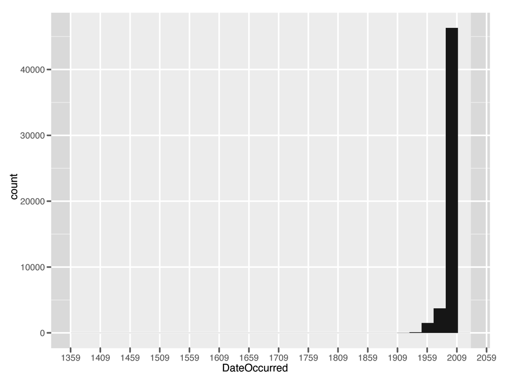
The results of this analysis are stark. The vast majority of
the data occur between 1960 and 2010, with the majority of UFO
sightings occurring within the last two decades. For our purposes,
therefore, we will focus on only those sightings that occurred
between 1990 and 2010. This will allow us to exclude the outliers
and compare relatively similar units during the analysis.
As before, we will use the subset function to create a new data frame
that meets this criteria:
ufo.us<-subset(ufo.us, DateOccurred>=as.Date("1990-01-01"))
nrow(ufo.us)
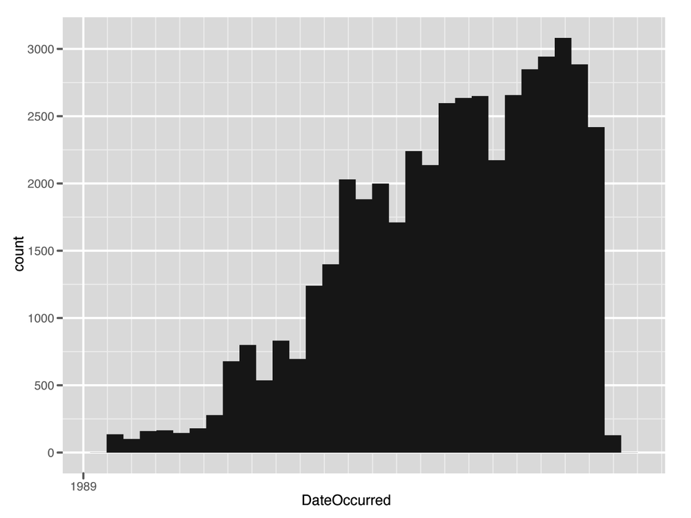
#[1] 46347Although this removes many more entries than we eliminated
while cleaning the data, it still leaves us with over 46,000
observations to analyze. To see the difference, we regenerate the
histogram of the subset data in Figure 1-6. We see that
there is much more variation when looking at this sample. Next, we
must begin organizing the data such that it can be used to address
our central question: what, if any, seasonal variation exists for
UFO sightings in US states? To address this, we must first ask: what
do we mean by “seasonal?” There are many ways to aggregate time
series data with respect to seasons: by week, month, quarter, year,
etc. But which way of aggregating our data is most appropriate here?
The DateOccurred column provides
UFO sighting information by the day, but there is considerable
inconsistency in terms of the coverage throughout the entire set. We
need to aggregate the data in a way that puts the amount of data for
each state on relatively level planes. In this case, doing so by
year-month is the best option. This aggregation also best addresses
the core of our question, as monthly aggregation will give good
insight into seasonal variations.
We need to count the number of UFO sightings that occurred in
each state by all year-month combinations from 1990–2010. First, we
will need to create a new column in the data that corresponds to the
years and months present in the data. We will use the strftime function to convert the Date objects to a string of the “YYYY-MM”
format. As before, we will set the format parameter accordingly to get the
strings:
ufo.us$YearMonth<-strftime(ufo.us$DateOccurred, format="%Y-%m")
Notice that in this case we did not use the transform function to add a new column to
the data frame. Rather, we simply referenced a column name that did
not exist, and R automatically added it. Both methods for adding new
columns to a data frame are useful, and we will switch between them
depending on the particular task. Next, we want to count the number
of times each state and year-month combination occurs in the data.
For the first time we will use the ddply function, which is part of the
extremely useful plyr library for
manipulating data.
The plyr family of
functions work a bit like the map-reduce-style data aggregation
tools that have risen in popularity over the past several years.
They attempt to group data in some specific way that was meaningful
to all observations, and then do some calculation on each of these
groups and return the results. For this task we want to group the
data by state abbreviations and the year-month column we just
created. Once the data is grouped as such, we count the number of
entries in each group and return that as a new column.
Here we will simply use the nrow function to reduce the data by the
number of rows in each group:
sightings.counts<-ddply(ufo.us,.(USState,YearMonth), nrow)
head(sightings.counts)
USState YearMonth V1
1      ak   1990-01  1
2      ak   1990-03  1
3      ak   1990-05  1
4      ak   1993-11  1
5      ak   1994-11  1
6      ak   1995-01  1
We now have the number of UFO sightings for each state by the
year and month. From the head
call in the example, however, we can see that there may be a problem
with using the data as is because it contains a lot of missing
values. For example, we see that there was one UFO sighting in
January, March, and May of 1990 in Alaska, but no entries appear for
February and April. Presumably, there were no UFO sightings in these
months, but the data does not include entries for nonsightings, so
we have to go back and add these as zeros.
We need a vector of years and months that spans the entire
data set. From this we can check to see whether they are already in
the data, and if not, add them as zeros. To do this, we will create a sequence of dates using the
seq.Date function, and then
format them to match the data in our data frame:
date.range<-seq.Date(from=as.Date(min(ufo.us$DateOccurred)),
                     to=as.Date(max(ufo.us$DateOccurred)), by="month")
date.strings<-strftime(date.range, "%Y-%m")
With the new date.strings
vector, we need to create a new data frame that has all year-months
and states. We will use this to perform the matching with the UFO
sighting data. As before, we will use the lapply function to create the columns and
the do.call function to convert
this to a matrix and then a data frame:
states.dates<-lapply(us.states,function(s) cbind(s,date.strings))
states.dates<-data.frame(do.call(rbind, states.dates), stringsAsFactors=FALSE)
head(states.dates)
s date.strings
1 ak      1990-01
2 ak      1990-02
3 ak      1990-03
4 ak      1990-04
5 ak      1990-05
6 ak      1990-06
The states.dates data frame
now contains entries for every year, month, and state combination
possible in the data. Note that there are now entries from February
and March 1990 for Alaska. To add in the missing zeros to the UFO
sighting data, we need to merge this data with our original data
frame. To do this, we will use the merge function, which takes two ordered
data frames and attempts to merge them by common columns. In our
case, we have two data frames ordered alphabetically by US state
abbreviations and chronologically by year and month. We need to tell
the function which columns to merge these data frames by. We will
set the by.x and by.y parameters according to the matching
column names in each data frame. Finally, we set the all parameter to TRUE, which instructs the function to
include entries that do not match and to fill them with NA. Those entries in the V1 column will be those state, year, and
month entries for which no UFOs were sighted:
all.sightings<-merge(states.dates,sightings.counts,by.x=c("s","date.strings"),
     by.y=c("USState","YearMonth"),all=TRUE)
head(all.sightings)
  s  date.strings V1
1 ak      1990-01  1
2 ak      1990-02 NA
3 ak      1990-03  1
4 ak      1990-04 NA
5 ak      1990-05  1
6 ak      1990-06 NA
The final steps for data aggregation are simple housekeeping.
First, we will set the column names in the new all.sightings data frame to something
meaningful. This is done in exactly the same way as we did it at the
outset. Next, we will convert the NA entries to zeros, again using the
is.na function. Finally, we will
convert the YearMonth and
State columns to the appropriate
types. Using the date.range
vector we created in the previous step and the rep function to create a new vector that
repeats a given vector, we replace the year and month strings with
the appropriate Date object.
Again, it is better to keep dates as Date objects rather than strings because
we can compare Date objects
mathematically, but we can’t do that easily with strings. Likewise,
the state abbreviations are better represented as categorical
variables than strings, so we convert these to factor types. We will describe factors and other R data types in more
detail in the next chapter:
names(all.sightings)<-c("State","YearMonth","Sightings")
all.sightings$Sightings[is.na(all.sightings$Sightings)]<-0
all.sightings$YearMonth<-as.Date(rep(date.range,length(us.states)))
all.sightings$State<-as.factor(toupper(all.sightings$State))For this data, we will address the core question only by
analyzing it visually. For the remainder of the book, we will
combine both numeric and visual analyses, but as this example is
only meant to introduce core R programming paradigms, we will stop
at the visual component. Unlike the previous histogram visualization, however, we
will take greater care with ggplot2 to build the visual layers
explicitly. This will allow us to create a visualization that
directly addresses the question of seasonal variation among states
over time and produce a more professional-looking
visualization.
We will construct the visualization all at once in the following example, then explain each layer individually:
state.plot<-ggplot(all.sightings, aes(x=YearMonth,y=Sightings))+
     geom_line(aes(color="darkblue"))+
     facet_wrap(~State,nrow=10,ncol=5)+
     theme_bw()+
     scale_color_manual(values=c("darkblue"="darkblue"),legend=FALSE)+
     scale_x_date(major="5 years", format="%Y")+
     xlab("Time")+ylab("Number of Sightings")+
     opts(title="Number of UFO sightings by Month-Year and U.S. State (1990-2010)")
ggsave(plot=state.plot, filename="../images/ufo_sightings.pdf",width=14,height=8.5)
As always, the first step is to create a ggplot object with a data frame as its
first argument. Here we are using the all.sightings data frame we created in the
previous step. Again, we need to build an aesthetic layer of data to
plot, and in this case the x-axis is the YearMonth column and the y-axis is the
Sightings data. Next, to show
seasonal variation among states, we will plot a line for each state.
This will allow us to observe any spikes, lulls, or oscillation in
the number of UFO sightings for each state over time. To do this, we will use the geom_line function and set the color to "darkblue" to
make the visualization easier to read.
As we have seen throughout this case, the UFO data is fairly
rich and includes many sightings across the United States over a
long period of time. Knowing this, we need to think of a way to
break up this visualization such that we can observe the data for
each state, but also compare it to the other states. If we plot all
of the data in a single panel, it will be very difficult to discern
variation. To check this, run the first line of code from the
preceding block, but replace color="darkblue" with color=State and enter >
print(state.plot) at the console. A better
approach would be to plot the data for each state individually and
order them in a grid for easy comparison.
To create a multifaceted plot, we use the facet_wrap function and specify that the
panels be created by the State
variable, which is already a factor type, i.e., categorical. We also
explicitly define the number of rows and columns in the grid, which
is easier in our case because we know we are creating 50 different
plots.
The ggplot2 package
has many plotting themes. The default theme is the one we used in
the first example and has a gray background with dark gray
gridlines. Although it is strictly a matter of taste, we prefer
using a white background for this plot because that will make it
easier to see slight differences among data points in our
visualization. We add the theme_bw layer, which will produce a plot
with a white background and black gridlines. Once you become more
comfortable with ggplot2, we
recommend experimenting with different defaults to find the one you
prefer.[5]
The remaining layers are done as housekeeping to make sure the
visualization has a professional look and feel. Though not formally
required, paying attention to these details is what can separate
amateurish plots from professional-looking data visualizations.
The scale_color_manual
function is used to specify that the string “darkblue” corresponds
to the web-safe color “darkblue.” Although this may seem repetitive,
it is at the core of ggplot2’s
design, which requires explicit definition of details such as color.
In fact, ggplot2 tends to think
of colors as a way of distinguishing among different types or
categories of data and, as such, prefers to have a factor type used to specify color. In our
case we are defining a color explicitly using a string and therefore
have to define the value of that string with the scale_color_manual function.
As we did before, we use the scale_x_date to specify the major
gridlines in the visualization. Because this data spans 20 years, we
will set these to be at regular five-year intervals. Then we set the
tick labels to be the year in a full four-digit format. Next,
we set the x-axis label to “Time” and the y-axis label
to “Number of Sightings” by using the xlab and ylab functions, respectively. Finally,
we use the opts
function to give the plot a title.There are many more options
available in the opts function,
and we will see some of them in later chapters, but there are many
more that are beyond the scope of this book.
With all of the layers built, we are now ready to render
the image with ggsave and analyze
the data.
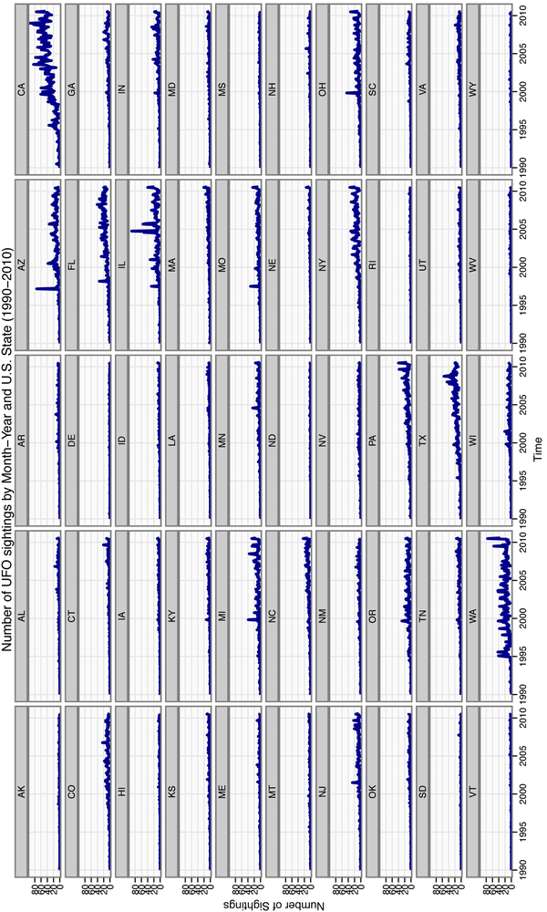
There are many interesting observations that fall out of this analysis (see Figure 1-7). We see that California and Washington are large outliers in terms of the number of UFO sightings in these states compared to the others. Between these outliers, there are also interesting differences. In California, the number of reported UFO sightings seems to be somewhat random over time, but steadily increasing since 1995, whereas in Washington, the seasonal variation seems to be very consistent over time, with regular peaks and valleys in UFO sightings starting from about 1995.
We can also notice that many states experience sudden spikes in the number of UFO sightings reported. For example, Arizona, Florida, Illinois, and Montana seem to have experienced spikes around mid-1997, and Michigan, Ohio, and Oregon experienced similar spikes in late-1999. Only Michigan and Ohio are geographically close among these groups. If we do not believe that these are actually the result of extraterrestrial visitors, what are some alternative explanations? Perhaps there was increased vigilance among citizens to look to the sky as the millennium came to a close, causing heavier reporting of false sightings.
If, however, you are sympathetic to the notion that we may be regularly hosting visitors from outer space, there is also evidence to pique your curiosity. In fact, there is surprising regularity of these sightings in many states in the US, with evidence of regional clustering as well. It is almost as if the sightings really contain a meaningful pattern.
This introductory case is by no means meant to be an exhaustive review of the language. Rather, we used this data set to introduce several R paradigms related to loading, cleaning, organizing, and analyzing data. We will revisit many of these functions and processes in the following chapters, along with many others. For those readers interested in gaining more practice and familiarity with R before proceeding, there are many excellent resources. These resources can roughly be divided into either reference books and texts or online resources, as shown in Table 1-3.
In the next chapter, we review exploratory data analysis. Much of the case study in this chapter involved exploring data, but we moved through these steps rather quickly. In the next chapter we will consider the process of data exploration much more deliberately.
Table 1-3. R references
| Title | Author | Reference | Description |
|---|---|---|---|
| Text references | |||
| Data Manipulation with R | Phil Spector | Spe08 | A deeper review of many of the data manipulation topics covered in the previous section, and an introduction to several techniques not covered. |
| R in a Nutshell | Joseph Adler | Adl10 | A detailed exploration of all of R’s base functions. This book takes the R manual and adds several practical examples. |
| Introduction to Scientific Programming and Simulation Using R | Owen Jones, Robert Maillardet, and Andrew Robinson | JMR09 | Unlike other introductory texts to R, this book focuses on the primacy of learning the language first, then creating simulations. |
| Data Analysis Using Regression and Multilevel/Hierarchical Models | Andrew Gelman and Jennifer Hill | GH06 | This text is heavily focused on doing statistical analyses, but all of the examples are in R, and it is an excellent resource for learning both the language and methods. |
| ggplot2: Elegant Graphics for Data Analysis | Hadley Wickham | Wic09 | The definitive guide to creating data
visualizations with ggplot2. |
| Online references | |||
| An Introduction to R | Bill Venables and David Smith | http://cran.r-project.org/doc/manuals/R-intro.html | An extensive and ever-changing introduction to the language from the R Core Team. |
| The R Inferno | Patrick Burns | http://lib.stat.cmu.edu/S/Spoetry/Tutor/R_inferno.pdf | An excellent introduction to R for the experienced programmer. The abstract says it best: “If you are using R and you think you’re in hell, this is a map for you.” |
| R for Programmers | Norman Matloff | http://heather.cs.ucdavis.edu/~matloff/R/RProg.pdf | Similar to The R Inferno, this introduction is geared toward programmers with experience in other languages. |
| “The Split-Apply-Combine Strategy for Data Analysis” | Hadley Wickham | http://www.jstatsoft.org/v40/i01/paper | The author of plyr provides an excellent
introduction to the map-reduce paradigm in the context of his
tools, with many examples. |
| “R Data Analysis Examples” | UCLA Academic Technology Services | http://www.ats.ucla.edu/stat/r/dae/default.htm | A great “Rosetta Stone”-style introduction for those with experience in other statistical programming platforms, such as SAS, SPSS, and Stata. |
Get Machine Learning for Hackers now with the O’Reilly learning platform.
O’Reilly members experience books, live events, courses curated by job role, and more from O’Reilly and nearly 200 top publishers.

