Chapter 4. Numbers
This chapter begins our tour of the Python language. In Python, data takes the form of objects—either built-in objects that Python provides, or objects we create using Python and C tools. Since objects are the most fundamental notion in Python programming, we’ll start this chapter with a survey of Python’s built-in object types before concentrating on numbers.
Python Program Structure
By way of introduction, let’s first get a clear picture of how this chapter fits into the overall Python picture. From a more concrete perspective, Python programs can be decomposed into modules, statements, expressions, and objects, as follows:
We introduced the highest level of this hierarchy when we learned about modules in Chapter 3. This part’s chapters begin at the bottom, exploring both built-in objects, and the expressions you can code to use them.
Why Use Built-in Types?
If you’ve used lower-level languages such as C or C++, you know that much of your work centers on implementing objects—also known as data structures—to represent the components in your application’s domain. You need to lay out memory structures, manage memory allocation, implement search and access routines, and so on. These chores are about as tedious (and error prone) as they sound, and usually distract from your programs’ real goals.
In typical Python programs, most of this grunt work goes away. Because Python provides powerful object types as an intrinsic part of the language, there’s no need to code object implementations before you start solving problems. In fact, unless you have a need for special processing that built-in types don’t provide, you’re almost always better off using a built-in object instead of implementing your own. Here are some reasons why:
Built-in objects make simple programs easy to write. For simple tasks, built-in types are often all you need to represent the structure of problem domains. Because you get things such as collections (lists) and search tables (dictionaries) for free, you can use them immediately. You can get a lot of work done with Python’s built-in object types alone.
Python provides objects and supports extensions. In some ways, Python borrows both from languages that rely on built-in tools (e.g., LISP), and languages that rely on the programmer to provide tool implementations or frameworks of their own (e.g., C++). Although you can implement unique object types in Python, you don’t need to do so just to get started. Moreover, because Python’s built-ins are standard, they’re always the same; frameworks tend to differ from site to site.
Built-in objects are components of extensions. For more complex tasks you still may need to provide your own objects, using Python statements or C language interfaces. But as we’ll see in later parts, objects implemented manually are often built on top of built-in types such as lists and dictionaries. For instance, a stack data structure may be implemented as a class that manages a built-in list.
Built-in objects are often more efficient than custom data structures. Python’s built-in types employ already optimized data structure algorithms that are implemented in C for speed. Although you can write similar object types on your own, you’ll usually be hard-pressed to get the level of performance built-in object types provide.
In other words, not only do built-in object types make programming easier, they’re also more powerful and efficient than most of what can be created from scratch. Regardless of whether you implement new object types or not, built-in objects form the core of every Python program.
Table 4-1 previews the built-in object types and some of the syntax used to code their literals— expressions that generate objects.[1] Some of these types will probably seem familiar if you’ve used other languages. For instance, numbers and strings represent numeric and textual values, respectively, and files provide an interface for processing files stored on your computer.
The object types in Table 4-1 are more general and powerful than what you may be accustomed to. For instance, you’ll find that lists and dictionaries obviate most of the work you do to support collections and searching in lower-level languages. Lists are ordered collections of other objects, and indexed by positions that start at 0. Dictionaries are collections of other objects that are indexed by key instead of position. Both dictionaries and lists may be nested, can grow and shrink on demand, and may contain objects of any type. For the full story, though, you’ll have to read on.
Numbers
The first object type on the tour is Python numbers. In general, Python’s number types are fairly typical and will seem familiar if you’ve used almost any other programming language in the past. They can be used to keep track of your bank balance, the distance to Mars, the number of visitors to your web site, and just about any other numeric quantity.
Python supports the usual numeric types (known as integer and floating point), as well as literals for creating numbers, and expressions for processing them. In addition, Python provides more advanced numeric programming support, including a complex number type, an unlimited precision integer, and a variety of numeric tool libraries. The next few sections give an overview of the numeric support in Python.
Number Literals
Among its basic types, Python supports the usual numeric types: both integer and floating-point numbers, and all their associated syntax and operations. Like the C language, Python also allows you to write integers using hexadecimal and octal literals. Unlike C, Python also has a complex number type, as well as a long integer type with unlimited precision (it can grow to have as many digits as your memory space allows). Table 4-2 shows what Python’s numeric types look like when written out in a program (that is, as literals).
|
Literal |
Interpretation |
|
|
Normal integers (C longs) |
|
|
Long integers (unlimited size) |
|
|
Floating-point (C doubles) |
|
|
Octal and hex literals |
|
|
Complex number literals |
In general, Python’s numeric types are straightforward, but a few coding concepts are worth highlighting here:
- Integer and floating-point literals
Integers are written as a string of decimal digits. Floating-point numbers have an embedded decimal point, and/or an optional signed exponent introduced by an
eorE. If you write a number with a decimal point or exponent, Python makes it a floating-point object and uses floating-point (not integer) math when it’s used in an expression. The rules for writing floating-point numbers are the same as in the C language.- Numeric precision and long integers
Plain Python integers (row 1 of Table 4-2) are implemented as C “longs” internally (i.e., at least 32 bits), and Python floating-point numbers are implemented as C “doubles”; Python numbers get as much precision as the C compiler used to build the Python interpreter gives to longs and doubles.[2]
- Long integer literals
On the other hand, if an integer literal ends with an
lorL, it becomes a Python long integer (not to be confused with a C long) and can grow as large as needed. In Python 2.2, because integers are converted to long integers on overflow, the letterLis no longer strictly required.- H exadecimal and octal literals
The rules for writing hexadecimal (base 16) and octal (base 8) integers are the same as in C. Octal literals start with a leading zero (
0), followed by a string of digits0-7; hexadecimals start with a leading0xor0X, followed by hexadecimal digits0-9, andA-F. In hexadecimal literals, hex digits may be coded in lower- or uppercase.- Complex numbers
Python complex literals are written as
realpart+imaginarypart, where theimaginarypartis terminated with ajorJ. Therealpartis technically optional, and theimaginarypartcan come first. Internally, they are implemented as a pair of floating-point numbers, but all numeric operations perform complex math when applied to complex numbers.
Built-in Tools and Extensions
Besides the built-in number literals shown in Table 4-2, Python provides a set of tools for processing number objects:
- Expression operators
+,*,>>,**, etc.- Built-in mathematical functions
pow,abs, etc.- Utility modules
random,math, etc.
We’ll meet all of these as we go along. Finally, if you need to do serious number-crunching, an optional extension for Python called NumPy (Numeric Python) provides advanced numeric programming tools, such as a matrix data type and sophisticated computation libraries. Hardcore scientific programming groups at places like Lawrence Livermore and NASA use Python with NumPy to implement the sorts of tasks they previously coded in C++ or FORTRAN.
Because it’s so advanced, we won’t say more about NumPy in this chapter. (See the examples in Chapter 29.) You will find additional support for advanced numeric programming in Python at the Vaults of Parnassus site. Also note that NumPy is currently an optional extension; it doesn’t come with Python and must be installed separately.
Python Expression Operators
Perhaps the most fundamental tool that processes numbers is the
expression:
a combination of numbers (or other objects) and operators that
computes a value when executed by Python. In Python, expressions are
written using the usual mathematical notation and operator symbols.
For instance, to add two numbers X and
Y, say X+Y, which tells Python
to apply the + operator to the values named by
X and Y. The result of the
expression is the sum of X and
Y, another number object.
Table 4-3 lists all the operator expressions
available in Python. Many are self-explanatory; for instance, the
usual mathematical operators are supported: +,
-, *,
/, and so on. A few will be familiar if
you’ve used C in the past: %
computes a division remainder, << performs a
bitwise left-shift, & computes a bitwise and
result, etc. Others are more Python-specific, and not all are numeric
in nature: the is operator tests object identity
(i.e., address) equality, lambda creates unnamed
functions, and so on. More on some of these later.
|
Operators |
Description |
|
|
Anonymous function generation |
|
Logical or (y is evaluated only if x is false) | |
|
|
Logical and (y is evaluated only if x is true) |
|
|
Logical negation |
|
|
Comparison operators, value equality operators, object identity tests, and sequence membership |
|
Bitwise or | |
|
|
Bitwise exclusive or |
|
|
Bitwise and |
|
Shift x left or right by y bits | |
|
|
Addition/concatenation, subtraction |
|
Multiplication/repetition, remainder/format, division[3] | |
|
Unary negation, identity, bitwise complement; binary power | |
|
|
Indexing, slicing, qualification, function calls |
|
| |
[3] Floor division ( [4] Beginning with Python 2.0, the list
syntax ( [5] Conversion of objects to their print strings
can also be accomplished with the more readable
| |
Mixed Operators: Operator Precedence
As in most languages, more complex expressions are coded by stringing together the operator expressions in Table 4-3. For instance, the sum of two multiplications might be written as a mix of variables and operators:
A * B + C * D
So how does Python know which operator to perform first? The solution to this lies in operator precedence. When you write an expression with more than one operator, Python groups its parts according to what are called precedence rules, and this grouping determines the order in which expression parts are computed. In Table 4-3, operators lower in the table have higher precedence and so bind more tightly in mixed expressions.
For example, if you write X + Y * Z, Python
evaluates the multiplication first (Y * Z), then
adds that result to X, because
* has higher precedence (is lower in the table)
than +. Similarly, in this
section’s original example, both multiplications
(A * B and C
*
D
) will happen before their results are added.
Parentheses Group Subexpressions
You can forget about precedence completely if you’re careful to group parts of expressions with parentheses. When you enclose subexpressions in parentheses, you override Python precedence rules; Python always evaluates expressions in parentheses first, before using their results in the enclosing expressions.
For instance, instead of coding X + Y * Z, write
one of the following to force Python evaluate the expression in the
desired order:
(X + Y) * Z
X + (Y * Z)
In the first case, + is applied to
X and Y first, because it is
wrapped in parentheses. In the second cases, the *
is performed first (just as if there were no parentheses at all).
Generally speaking, adding parentheses in big expressions is a great
idea; it not only forces the evaluation order you want, but it also
aids readability.
Mixed Types: Converted Up
Besides mixing operators in expressions, you can also mix numeric types. For instance, you can add an integer to a floating-point number:
40 + 3.14
But this leads to another question: what type is the result—integer or floating-point? The answer is simple, especially if you’ve used almost any other language before: in mixed type expressions, Python first converts operands up to the type of the most complicated operand, and then performs the math on same-type operands. If you’ve used C, you’ll find this similar to type conversions in that language.
Python ranks the complexity of numeric types like so: integers are simpler than long integers, which are simpler than floating-point numbers, which are simpler than complex numbers. So, when an integer is mixed with a floating-point, as in the example, the integer is converted up to a floating-point value first, and floating-point math yields the floating-point result. Similarly, any mixed-type expression where one operand is a complex number results in the other operand being converted up to a complex number that yields a complex result.
As you’ll see later in this section, as of Python 2.2, Python also automatically converts normal integers to long integers, whenever their values are too large to fit in a normal integer. Also keep in mind that all these mixed type conversions only apply when mixing numeric types around an operator or comparison (e.g., an integer and a floating-point number). In general, Python does not convert across other type boundaries. Adding a string to an integer, for example, results in an error, unless you manually convert one or the other; watch for an example when we meet strings in Chapter 5.
Preview: Operator Overloading
Although we’re focusing on
built-in
numbers
right now,
keep in mind that all Python operators may be overloaded (i.e.,
implemented) by Python classes and C extension types, to work on
objects you create. For instance, you’ll see later
that objects coded with classes may be added with
+ expressions, indexed with [i]
expressions, and so on.
Furthermore, some operators are already overloaded by Python itself;
they perform different actions depending on the type of built-in
objects being processed. For example, the +
operator performs addition when applied to numbers, but performs
concatenation when applied to sequence objects such as strings and
lists.[6]
Numbers in Action
Probably the best way to understand numeric objects and expressions is to see them in action. So, start up the interactive command line and type some basic, but illustrative operations.
Basic Operations and Variables
First of all, let’s exercise some basic math. In the
following interaction, we first assign two
variables
(a and b) to integers, so we
can use them later in a larger expression. Variables are simply
names—created by you or Python—that are used to keep
track of information in your program. We’ll say more
about this later, but in Python:
Variables are created when first assigned a value.
Variables are replaced with their values when used in expressions.
Variables must be assigned before they can be used in expressions.
Variables refer to objects, and are never declared ahead of time.
In other words, the assignments cause these variables to spring into existence automatically.
%python>>>a = 3 # Name created>>>b = 4
We’ve also used a
comment
here. In Python code, text after a # mark and
continuing to the end of the line is considered to be a comment, and
is ignored by Python. Comments are a place to write human-readable
documentation for your code. Since code you type interactively is
temporary, you won’t normally write comments there,
but they are added to examples to help explain the code.[7] In the next part of this book,
we’ll meet a related feature—documentation
strings—that attaches the text of your comments to objects.
Now, let’s use the integer objects in expressions.
At this point, a and b are
still 3 and 4, respectively; variables like these are replaced with
their values whenever used inside an expression, and expression
results are echoed back when working interactively:
>>>a + 1, a - 1 # Addition (3+1), subtraction (3-1)(4, 2)>>>b * 3, b / 2 # Multiplication (4*3), division (4/2)(12, 2)>>>a % 2, b ** 2 # Modulus (remainder), power(1, 16)>>>2 + 4.0, 2.0 ** b # Mixed-type conversions(6.0, 16.0)
Technically, the results being echoed back here are
tuples of two values, because lines typed at the
prompt contain two expressions separated by commas;
that’s why the result are displayed in parenthesis
(more on tuples later). Notice that the expressions work because the
variables a and b within them
have been assigned values; if you use a different variable that has
never been assigned, Python reports an error rather than filling in
some default value:
>>> c * 2
Traceback (most recent call last):
  File "<stdin>", line 1, in ?
NameError: name 'c' is not defined
You don’t need to predeclare variables in Python, but they must be assigned at least once before you can use them at all. Here are two slightly larger expressions to illustrate operator grouping and more about conversions:
>>>b / 2 + a # Same as ((4 / 2) + 3)5 >>>print b / (2.0 + a) # Same as (4 / (2.0 + 3))0.8
In the first expression, there are no parentheses, so Python
automatically groups the components according to its precedence
rules—since / is lower in Table 4-3 than +, it binds more
tightly, and so is evaluated first. The result is as if the
expression had parenthesis as shown in the comment to the right of
the code. Also notice that all the numbers are integers in the first
expression; because of that, Python performs integer division and
addition.
In the second expression, parentheses are added around the
+ part to force Python to evaluate it first (i.e.,
before the /). We also made one of the operands
floating-point by adding a decimal point: 2.0.
Because of the mixed types, Python converts the integer referenced by
a to a floating-point value
(3.0) before performing the +.
It also converts b to a floating-point value
(4.0) and performs a floating-point division;
(4.0/5.0) yields a floating-point result of
0.8. If all the numbers in this expression were
integers, it would invoke integer division (4/5),
and the result would be the truncated integer 0
(in Python 2.2, at least—see the discussion of true division
ahead).
Numeric Representation
By the way, notice that we
used a
print statement in the second example; without the
print, you’ll see something that
may look a bit odd at first glance:
>>>b / (2.0 + a) # Auto echo output: more digits0.80000000000000004 >>>print b / (2.0 + a) # print rounds off digits.0.8
The whole story behind this has to do with the limitations of
floating-point hardware, and its inability to exactly represent some
values. Since computer architecture is well beyond this
book’s scope, though, we’ll finesse
this by saying that all of the digits in the first output are really
there, in your computer’s floating-point hardware;
it’s just that you’re not normally
accustomed to seeing them. We’re using this example
to demonstrate the difference in output formatting—the
interactive prompt’s automatic result echo shows
more digits than the print statement. If you
don’t want all the digits, say
print.
Note that not all values have so many digits to display:
>>> 1 / 2.0
0.5
And there are more ways to display the bits of a number inside your computer than prints and automatic echoes:
>>>num = 1 / 3.0>>>num # Echoes0.33333333333333331 >>>print num # Print rounds0.333333333333 >>>"%e" % num # String formatting'3.333333e-001' >>>"%2.2f" % num # String formatting'0.33'
The last two of these employ string formatting—an expression that allows for format flexibility, explored in the upcoming chapter on strings.
Division: Classic, Floor, and True
Now that you’ve seen how division works, you should know that it is scheduled for a slight change in a future Python release (currently, in 3.0, scheduled to appear years after this edition is released). In Python 2.3, things work as just described, but there are actually two different division operators, one of which will change:
-
X / Y Classic division. In Python 2.3 and earlier, this operator truncates results down for integers, and keeps remainders for floating-point numbers, as described here. This operator will be changed to true division—always keeping remainders regardless of types—in a future Python release (3.0).
-
X // Y Floor division. Added in Python 2.2, this operator always truncates fractional remainders down to their floor, regardless of types.
Floor division was added to address the fact that the result of the current classic division model is dependent on operand types, and so can sometimes be difficult to anticipate in a dynamically-typed language like Python.
Due to possible backward compatibility issues, this is in a state of
flux today. In version 2.3, / division works as
described by default, and // floor division has
been added to truncate result remainders to their floor regardless of
types:
>>>(5 / 2), (5 / 2.0), (5 / -2.0), (5 / -2)(2, 2.5, -2.5, -3) >>>(5 // 2), (5 // 2.0), (5 // -2.0), (5 // -2)(2, 2.0, -3.0, -3) >>>(9 / 3), (9.0 / 3), (9 // 3), (9 // 3.0)(3, 3.0, 3, 3.0)
In a future Python release, / division will likely
be changed to return a true division result which always retains
remainders, even for integers—for example,
1/2 will be 0.5, not
0, and 1//2 will still be
0.
Until this change is incorporated completely, you can see the way
that the / will likely work in the future, by
using a special import of the form: from __future__
import division. This turns the
/ operator into a true division (keeping
remainders), but leaves // as is.
Here’s how / will eventually
behave:
>>>from __future__ import division>>>(5 / 2), (5 / 2.0), (5 / -2.0), (5 / -2)(2.5, 2.5, -2.5, -2.5) >>>(5 // 2), (5 // 2.0), (5 // -2.0), (5 // -2)(2, 2.0, -3.0, -3) >>>(9 / 3), (9.0 / 3), (9 // 3), (9 // 3.0)(3.0, 3.0, 3, 3.0)
Watch for a simple prime number while loop example
in Chapter 10, and a corresponding exercise at the
end of Part IV, which illustrate the sort of
code that may be impacted by this / change. In
general, any code that depends on / truncating an
integer result may be effected (use the new //
instead). As we write this, this change is scheduled to occur in
Python 3.0, but be sure to try these expressions in your version to
see which behavior applies. Also stay tuned for more on the special
from command used here in Chapter 18.
B itwise Operations
Besides the normal numeric operations (addition, subtraction, and so on), Python supports most of the numeric expressions available in the C language. For instance, here it’s at work performing bitwise shift and Boolean operations:
>>>x = 1 # 0001>>>x << 2 # Shift left 2 bits: 01004 >>>x | 2 # bitwise OR: 00113 >>>x & 1 # bitwise AND: 00011
In the first expression, a binary 1 (in base 2,
0001) is shifted left two slots to create a binary
4 (0100). The last two
operations perform a binary or
(0001|0010 = 0011), and a
binary and (0001&0001 =
0001). Such bit masking operations allow us to
encode multiple flags and other values within a single integer.
We won’t go into much more detail on “bit-twiddling” here. It’s supported if you need it, but be aware that it’s often not as important in a high-level language such as Python as it is in a low-level language such as C. As a rule of thumb, if you find yourself wanting to flip bits in Python, you should think about which language you’re really coding. In general, there are often better ways to encode information in Python than bit strings.[8]
L ong Integers
Now for something more exotic: here’s a look at long
integers in action. When an integer literal ends with a letter
L (or lowercase l), Python
creates a long integer. In Python, a long integer can be arbitrarily
big—it can have as many digits as you have room for in
memory:
>>> 9999999999999999999999999999999999999L + 1
10000000000000000000000000000000000000L
The L at the end of the digit string tells Python
to create a long integer object with unlimited precision. As of
Python 2.2, even the letter L is largely
optional—Python automatically converts normal integers up to
long integers, whenever they overflow normal integer precision
(usually 32 bits):
>>> 9999999999999999999999999999999999999 + 1
10000000000000000000000000000000000000L
Long integers are a convenient built-in tool. For instance, you can use them to count the national debt in pennies in Python directly (if you are so inclined and have enough memory on your computer). They are also why we were able to raise 2 to such large powers in the examples of Chapter 3:
>>>2L ** 2001606938044258990275541962092341162602522202993782792835301376L >>> >>>2 ** 2001606938044258990275541962092341162602522202993782792835301376L
Because Python must do extra work to support their extended precision, long integer math is usually substantially slower than normal integer math (which usually maps directly to the hardware). If you need the precision, it’s built in for you to use; but there is a performance penalty.
A note on version skew: prior to Python 2.2, integers were not
automatically converted up to long integers on overflow, so you
really had to use the letter L to get the extended
precision:
>>>9999999999999999999999999999999999999 + 1 # Before 2.2OverflowError: integer literal too large >>>9999999999999999999999999999999999999L + 1 # Before 2.210000000000000000000000000000000000000L
In Version 2.2 the L is mostly optional. In the
future, it is possible that using the letter L may
generate a warning. Because of that, you are probably best off
letting Python convert up for you automatically when needed, and
omitting the L.
Complex Numbers
C
omplex numbers are a distinct core
object type in Python. If you know what they are, you know why they
are useful; if not, consider this section optional reading. Complex
numbers are represented as two floating-point numbers—the real
and imaginary parts—and are coded by adding a
j or J
suffix
to the imaginary part.
We can also write complex numbers with a nonzero real part by adding
the two parts with a +. For example, the complex
number with a real part of 2 and an imaginary part
of -3 is written: 2 + -3j. Here
are some examples of complex math at work:
>>>1j * 1J(-1+0j) >>>2 + 1j * 3(2+3j) >>>(2+1j)*3(6+3j)
Complex numbers also allow us to extract their parts as attributes,
support all the usual mathematical expressions, and may be processed
with tools in the standard cmath module (the
complex version of the standard math module).
Complex numbers typically find roles in engineering-oriented
programs. Since they are an advanced tool, check
Python’s language reference manual for additional
details.
Hexadecimal and Octal Notation
As mentioned at the start of this section, Python integers can be coded in hexadecimal (base 16) and octal (base 8) notation, in addition to the normal base 10 decimal coding:
Octal literals have a leading 0, followed by a string of octal digits 0-7, each of which represents 3 bits.
Hexadecimal literals have a leading 0x or 0X, followed by a string of hex digits 0-9 and upper- or lowercase A-F, each of which stands for 4 bits.
Keep in mind that this is simply an alternative syntax for specifying the value of an integer object. For example, the following octal and hexadecimal literals produce normal integers, with the specified values:
>>>01, 010, 0100 # Octal literals(1, 8, 64) >>>0x01, 0x10, 0xFF # Hex literals(1, 16, 255)
Here, the octal value 0100 is decimal
64, and hex 0xFF is decimal
255. Python prints in decimal by default, but
provides built-in functions that allow you to convert integers to
their octal and hexadecimal digit strings:
>>> oct(64), hex(64), hex(255)
('0100', '0x40', '0xff')
The oct function converts decimal to octal, and
hex to hexadecimal. To go the other way, the
built-in int function converts a string of digits
to an integer; an optional second argument lets you specify the
numeric base:
>>> int('0100'), int('0100', 8), int('0x40', 16)
(100, 64, 64)
The eval function, which you’ll
meet later in this book, treats strings as though they were Python
code. It therefore has a similar effect (but usually runs more
slowly—it actually compiles and runs the string as a piece of a
program):
>>> eval('100'), eval('0100'), eval('0x40')
(100, 64, 64)
Finally, you can also convert integers to octal and hexadecimal strings with a string formatting expression:
>>> "%o %x %X" % (64, 64, 255)
'100 40 FF'
This is covered in Chapter 4.
One warning before moving on, be careful to not begin a string of digits with a leading zero in Python, unless you really mean to code an octal value. Python will treat it as base 8, which may not work as you’d expect—010 is always decimal 8, not decimal 10 (despite what you might think!).
Other Numeric Tools
Python also provides
both
built-in functions and built-in
modules for numeric processing. Here are examples of the built-in
math module and a few built-in functions at work.
>>>import math>>>math.pi, math.e(3.1415926535897931, 2.7182818284590451) >>>math.sin(2 * math.pi / 180)0.034899496702500969 >>>abs(-42), 2**4, pow(2, 4)(42, 16, 16) >>>int(2.567), round(2.567), round(2.567, 2)(2, 3.0, 2.5699999999999998)
The math module contains most of the tools in the
C language’s math library. As described earlier, the
last output here will be just 2.57 if we say
print.
Notice that built-in modules such as math must be
imported, but built-in functions such as abs are
always available without imports. In other words, modules are
external components, but built-in functions live in an implied
namespace, which Python automatically searches to find names used in
your program. This namespace corresponds to the module called
__builtin__. There is much more about name
resolution in Part IV, Functions; for now, when you
hear
“module,” think
“import.”
The Dynamic Typing Interlude
If you have a background in compiled or statically-typed languages
like C, C++, or Java, you might find yourself in a perplexed place at
this point. So far, we’ve been using variables
without declaring their types—and it somehow works. When we
type a = 3 in an interactive session or program
file, how does Python know that a should stand for
an integer? For that matter, how does Python know what
a even is at all?
Once you start asking such questions, you’ve crossed over into the domain of Python’s dynamic typing model. In Python, types are determined automatically at runtime, not in response to declarations in your code. To you, it means that you never declare variables ahead of time, and that is perhaps a simpler concept if you have not programmed in other languages before. Since this is probably the most central concept of the language, though, let’s explore it in detail here.
How Assignments Work
You’ll notice that when we say a =
3, it works, even though we never told Python to use name
a as a variable.
In
addition, the assignment of 3 to
a seems to work too, even though we
didn’t tell Python that a should
stand for an integer type object. In the Python language, this all
pans out in a very natural way, as follows:
- Creation
A variable, like
a, is created when it is first assigned a value by your code. Future assignments change the already-created name to have a new value. Technically, Python detects some names before your code runs; but conceptually, you can think of it as though assignments make variables.- Types
A variable, like
a, never has any type information or constraint associated with it. Rather, the notion of type lives with objects, not names. Variables always simply refer to a particular object, at a particular point in time.- Use
When a variable appears in an expression, it is immediately replaced with the object that it currently refers to, whatever that may be. Further, all variables must be explicitly assigned before they can be used; use of unassigned variables results in an error.
This model is strikingly different from traditional languages, and is responsible for much of Python’s conciseness and flexibility. When you are first starting out, dynamic typing is usually easier to understand if you keep clear the distinction between names and objects. For example, when we say this:
>>> a = 3At least conceptually, Python will perform three distinct steps to carry out the request, which reflect the operation of all assignments in the Python language:
Create an object to represent the value
3.Create the variable
a, if it does not yet exist.Link the variable
ato the new object3.
The net result will be a structure inside Python that resembles Figure 4-1. As sketched, variables and objects are stored in different parts of memory, and associated by links—shown as a pointer in the figure. Variables always link to objects (never to other variables), but larger objects may link to other objects.
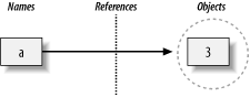
These links from variables to objects are called references in Python—a kind of association.[9] Whenever variables are later used (i.e., referenced), the variable-to-object links are automatically followed by Python. This is all simpler than its terminology may imply. In concrete terms:
Variables are simply entries in a search table, with space for a link to an object.
Objects are just pieces of allocated memory, with enough space to represent the value they stand for, and type tag information.
At least conceptually, each time you generate a new value in your
script, Python creates a new object (i.e., a chunk of memory) to
represent that value. Python caches and reuses certain kinds of
unchangeable objects like small integers and strings as an
optimization (each zero is not really a new piece of memory); but it
works as though each value is a distinct object.
We’ll revisit this concept when we meet the
== and is comparisons in Section 7.6 in Chapter 7.
Let’s extend the session and watch what happens to its names and objects:
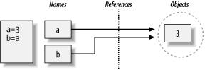
>>>a = 3>>>b = a
After typing these two statements, we generate the scene captured in
Figure 4-2. As before, the second line causes
Python to create variable b; variable
a is being used and not assigned here, so it is
replaced with the object it references (3); and
b is made to reference that object. The net effect
is that variables a and b wind
up referencing the same object (that is, pointing to the same chunk
of memory). This is called a shared reference in
Python—multiple names referencing the same object.
Next, suppose we extend the session with one more statement:
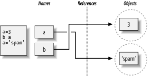
>>>a = 3>>>b = a>>>a = 'spam'
As for all Python assignments, this simply makes a new object to
represent the string value “spam”,
and sets a to reference this new object. It does
not, however, change the value of b; b still
refers to the original object, the integer 3. The
resulting reference structure is as in Figure 4-3.
The same sort of thing would happen if we changed
b to “spam”
instead—the assignment would only change b,
and not a. This example tends to look especially
odd to ex-C programmers—it seems as though the
type of a changed from
integer to string, by saying a = 'spam‘. But not
really. In Python, things work more simply: types live with objects,
not names. We simply change a to reference a
different object.
This behavior also occurs if there are no type differences at all. For example, consider these three statements:
>>>a = 3>>>b = a>>>a = 5
In this sequence, the same events transpire: Python makes variable
a reference the object 3, and
makes b reference the same object as
a, as in Figure 4-2. As before,
the last assignment only sets a to a completely
different object, integer 5. It does not change
b as a side effect. In fact, there is no way to
ever overwrite the value of object 3 (integers can
never be changed in place—a property called
immutability). Unlike some languages, Python
variables are always pointers to objects, not labels of changeable
memory areas.
References and Changeable Objects
As you’ll see later in this part’s chapters, though, there are objects and operations that perform in-place object changes. For instance, assignment to offsets in lists actually changes the list object itself (in-place), rather than generating a brand new object. For objects that support such in-place changes, you need to be more aware of shared references, since a change from one name may impact others. For instance, list objects support in-place assignment to positions:
>>>L1 = [2,3,4]>>>L2 = L1
As noted at the start of this chapter, lists are simply collections
of other objects, coded in square brackets; L1
here is a list containing objects 2,
3, and 4. Items inside a list
are accessed by their positions; L1[0] refers to
object 2, the first item in the list
L1.
Lists are also objects in their own right, just like integers and
strings. After running the two prior assignments,
L1 and L2 reference the same
object, just like the prior example (see Figure 4-2). Also as before, if we now say this:
>>> L1 = 24then L1 is simply set to a different object;
L2 is still the original list. If instead we
change this statement’s syntax slightly, however, it
has radically different effect:
>>>L1[0] = 24>>>L2[24, 3, 4]
Here, we’ve changed a component of the
object that L1 references,
rather than changing L1 itself. This sort of
change overwrites part of the list object in-place. The upshot is
that the effect shows up in L2 as well, because it
shares the same object as L1.
This is usually what you want, but you should be aware of how this works so that it’s expected. It’s also just the default: if you don’t want such behavior, you can request that Python copy objects, instead of making references. We’ll explore lists in more depth, and revisit the concept of shared references and copies, in Chapter 6 and Chapter 7.[10]
References and Garbage Collection
When names are made to reference new objects, Python also reclaims the old object, if it is not reference by any other name (or object). This automatic reclamation of objects’ space is known as garbage collection . This means that you can use objects liberally, without ever needing to free up space in your script. In practice, it eliminates a substantial amount of bookkeeping code compared to lower-level languages such as C and C++.
To illustrate, consider the following example, which sets name
x to a different object on each assignment. First
of all, notice how the name x is set to a
different type of object each time.
It’s as though the type of x is
changing over time; but not really, in Python, types live with
objects, not names. Because names are just generic references to
objects, this sort of code works naturally:
>>>x = 42>>>x = 'shrubbery' # Reclaim 42 now (?)>>>x = 3.1415 # Reclaim 'shrubbery' now (?)>>>x = [1,2,3] # Reclaim 3.1415 now (?)
Second of all, notice that references to objects
are discarded along the way. Each time x is
assigned to a new object, Python reclaims the prior object. For
instance, when x is assigned the string
'shrubbery', the object 42 will
be immediately reclaimed, as long as it is not referenced anywhere
else—the object’s space is automatically
thrown back into the free space pool, to be reused for a future
object.
Technically, this collection behavior may be more conceptual than
literal, for certain types. Because Python caches and reuses integers
and small strings as mentioned earlier, the object
42 is probably not literally reclaimed; it remains
to be reused the next time you generate a 42 in
your code. Most kinds of objects, though, are reclaimed immediately
when no longer referenced; for those that are not, the caching
mechanism is irrelevant to your code.
Of course, you don’t really need to draw name/object
diagrams with circles and arrows in order to use Python. When you are
starting out, though, it sometimes helps you understand some unusual
cases, if you can trace their reference structure. Moreover, because
everything seems to be assignment and references
in Python, a basic understanding of this model helps in many
contexts—as we’ll see, it works the same in
assignment statements, for loop variables,
function arguments, module imports,
and more.
[1] In this book, the term
literal simply means an expression whose syntax
generates an object—sometimes also called a
constant. If you hear these called constants, it
does not imply objects or variables that can never be changed (i.e.,
this is unrelated to C++’s const, or
Python’s
“immutable”—a topic explored
later in this part of the book).
[2] That is, the standard CPython implementation. In the Jython Java-based implementation, Python types are really Java classes.
[6] This is usually called polymorphism—the meaning of an operation depends on the type of objects being operated on. We’ll revisit this word when we explore functions in Chapter 12, because it becomes a much more obvious feature there.
[7] If you’re working along, you
don’t need to type any of the comment text from
# through the end of the line; comments are simply
ignored by Python, and not a required part of the statements we
run.
[8] As for most rules, there are exceptions. For instance, if you interface with C libraries that expect bit strings to be passed in, this doesn’t apply.
[9] Readers with a background in C may find Python references similar to C pointers (memory addresses). In fact, references are implemented as pointers, and often serve the same roles, especially with objects that can be changed in place (more on this later). However, because references are always automatically dereferenced when used, you can never actually do anything useful with a reference itself; this is a feature, which eliminates a vast category of C bugs. But, you can think of Python references as C “void*” pointers, which are automatically followed whenever used.
[10] Objects that can be changed in-place are known as mutables—lists and dictionaries are mutable built-ins, and hence susceptible to in-place change side-effects.
Get Learning Python, 2nd Edition now with the O’Reilly learning platform.
O’Reilly members experience books, live events, courses curated by job role, and more from O’Reilly and nearly 200 top publishers.

