VLSI Digital Signal Processing Systems: Design and Implementation

8.5    CYCLIC CONVOLUTION

Cyclic convolution is also known as circular convolution. Let h = {h₀, h₁,· · ·, h_n−1} be the filter coefficients and x = {x₀,x₁,· · ·,x_n−1} be the data sequence. The cyclic convolution can be expressed as

and the output samples are given by

where ((i–k)) denotes (i–k) mod n. The cyclic convolution can be computed as a linear convolution reduced by modulo pⁿ – 1. (Notice that there are 2n – 1 different output samples for this linear convolution). Alternatively, the cyclic convolution can be computed using CRT with m(p) = pⁿ – 1, which is much simpler.

Example 8.5.1 Construct a 4 × 4 cyclic convolution algorithm using CRT with m(p) = p⁴ – 1 = (p – 1)(p + 1)(p² + 1).

Solution

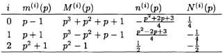
Let h(p) = h₀ + h₁p + h₂p² + h₃p³ and x(p) = x₀ + x₁p + x₂p² + x₃p³. Let m⁽⁰⁾(p) = p – 1, m⁽¹⁾(p) = p + 1, m⁽²⁾(p) = p² + 1. Let . Use the relationship (8.37) to construct the following table:

Compute residues

and

Notice that it takes 1 multiplication to compute and 1 to compute The computation ...