VLSI Digital Signal Processing Systems: Design and Implementation

12.9    DESIGN EXAMPLES OF PIPELINED LATTICE FILTERS

To pipeline basic, 1-multiplier, normalized, and scaled-normalized lattice filters by M levels, the denominator of a transfer function is required to have (M − 1) consecutive zero coefficients between each 2 nonzero coefficients of nearest degree. The pipelinable transfer functions can be obtained by applying the scattered look-ahead method to the nonpipelined filter transfer functions. To avoid the drawbacks of the cancelling zeros such as hardware increase and inexact pole-zero cancellations in a finite wordlength implementation, a pipelinable transfer function can also be designed directly from the filter spectrum while the denominator is constrained to be a polynomial in z^M rather than z.

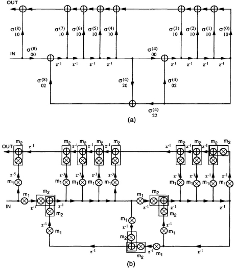
Fig. 12.31    (a) A 4-level pipelined normalized lattice filter before retiming.  (b) The 4-level pipelined normalized lattice filter after retiming. Computation_Time(m₁) = Computation_Time(m₂) = Computation_Time(multiply & add)/2.

In this section, two design examples of pipelined lattice filters are presented. The pipelinable transfer functions have been obtained by the modified Deczky’s method [19].

Example 12.9.1    Consider a 4-stage pipelinable low-pass filter with

pass-band: 0 − 0.2π (0.5 dB) and stop-band: 0.3π − π (20 dB).

The transfer function obtained by the modified Deczky’s method is:

Notice that D(z) can be further decomposed ...