Chapter 4. Variable-Length Codes
The examples in the previous chapter showed two things: we can save bits by encoding some symbols with fewer or more bits than others, and that this doesn’t work well when there are duplicate symbols in the data set. And let’s face it, real-life data sets are full of duplicates.
This, at its core, is why the LOG2 number system doesn’t properly represent the true information content of a data set. This chapter shows how you can do some nifty things based on probability and duplication that can yield impressive compression results.
Morse Code
To begin talking about transmitting real-life data, let’s go way back to the age of the telegraph and Morse code.
Beginning in 1836, American artist Samuel F. B. Morse, American physicist Joseph Henry, and American machinist Alfred Vail developed an electrical telegraph system. This system sent pulses of electric current1 along wires, and the pulses interacted with an electromagnet that was located at the receiving end of the telegraph system, creating audible taps, or, when a paper (ticker) tape was moved under the thing doing the tapping at a constant rate, a paper record of the signals received.
The telegraph was a fantastic invention in terms of being able to communicate human information across long distances. Eventually losing the wires (see Figure 4-1), it evolved into the mobile device in your pocket.
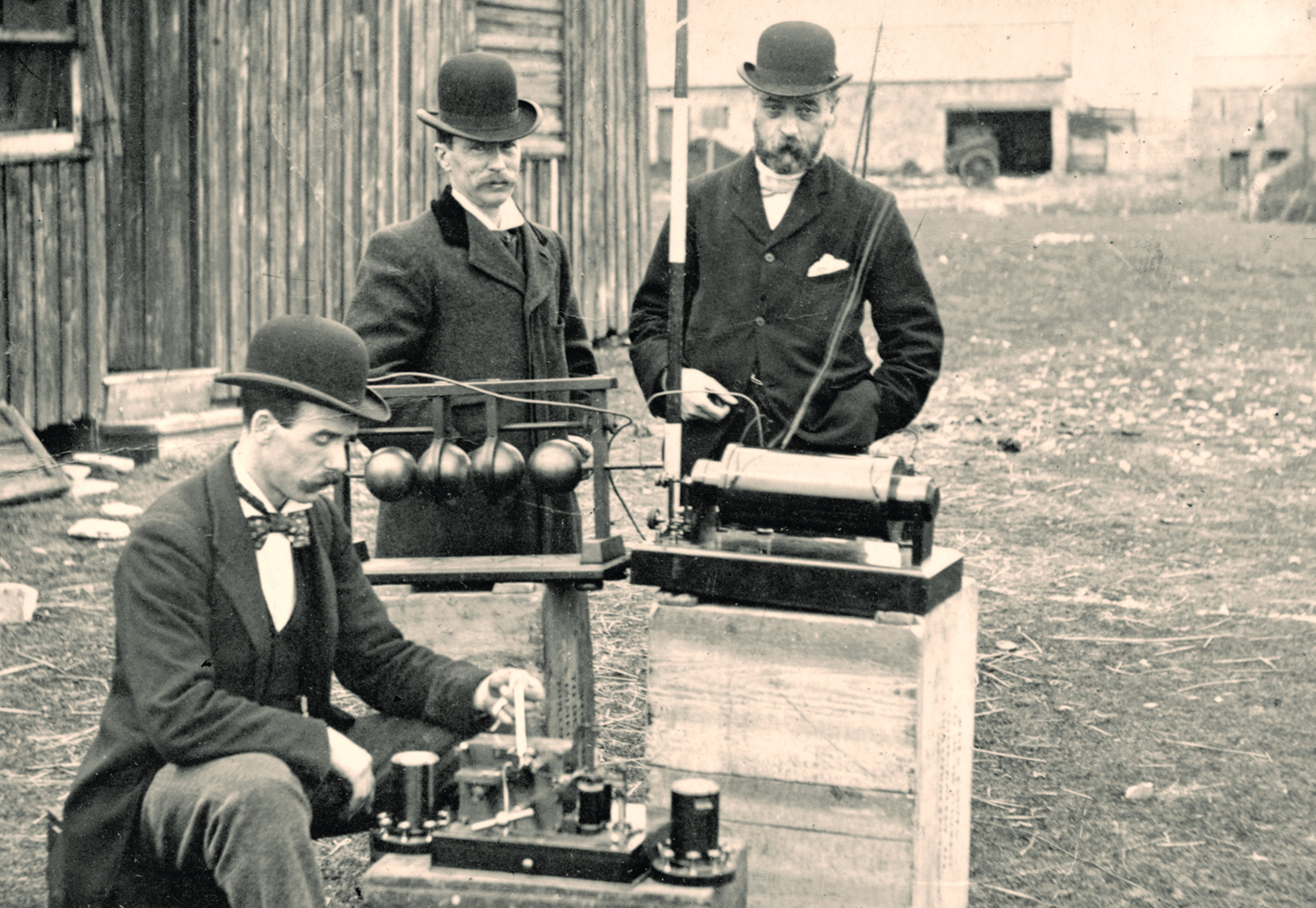
Figure 4-1. British post office engineers inspect Guglielmo Marconi’s wireless telegraphy equipment during a demonstration on Flat Holm island, May 13, 1897. This was the world’s first demonstration of the transmission of radio signals over open sea, between Lavernock Point and Flat Holm Island, a distance of three miles. Source: Wikipedia.
However, the developers now needed a way to represent human concepts, such as language, in a way that the signals of electric current could carry. The device itself worked very simplistically for the operator: push the telegraph key to make a connection and send current across the wire; leave the key up, and no current is sent. Even though binary code hadn’t been invented yet, back in the 1800s, this system was effectively using the same idea for communicating information.
Perhaps the simplest way to encode some text information would be to number all of the English characters—A to Z—with numeric values 0–26. You could then use the number of pulses, along with pairing, to determine what digit you were transmitting. For example, you could translate “THE HAT” into 20-8-5 8-1-20. In reality, the system would also need a way to determine the differences between words, spaces, punctuation, and eventually end-of-message, but you get the gist.
Remember, though, that these signals were transmitted by a human operator banging on a telegraph key. So, “THE HAT” would cost the same number of operator actions as “FAT CAT” and “TIP TOP.” This gets gets pretty crazy when you have a post office sending 100 to 200 telegrams of 50 words each, all day long. It quickly became apparent that the number of physical actions required to send a message was becoming too high. Physical hardware (the machine) and human hardware (the operator’s wrist) were wearing down faster than expected. The solution was to use statistics to reduce overall work. You see, some letters in the English language are used more frequently than others. For example, E is used 12% of the time, whereas G is used only 2% of the time. If the operator is going to be banging out more “E”s during the day, we should make those as fast and easy as possible, right?
And thus, Morse code was invented.
This system applied a set of long and short pulses to each character in the English alphabet; the more frequent the character, the smaller and simpler the code. Thus, the most common letter in English, the letter “E,” has the shortest code, a single dot, and “X” unsurprisingly is long-ish, and all numbers use five pulses. Figure 4-2 shows the original character set.
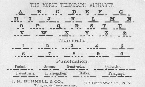
Figure 4-2. Morse code assigns dots and dashes to symbols based on their probability of occurrence in the English language. The more probable a symbol, the shorter its code. This image is an early version of Morse code, defined specifically by telegraph companies for transmitting small sets of information. Morse has evolved since then, and looks very different now.
Even back in the 1800s, this was one of the first realizations of assigning variable-length codes to symbols in order to reduce the overall amount of work that needed to be done to communicate a message.
It makes sense then that Claude Shannon (who was an expert in Morse code) would be able to take advantage of this concept in his early research of information theory to produce the first generation of a new field of technology, called “data compression,” all with the help of variable-length codes.
Probability, Entropy, and Codeword Size
For the sake of data compression, our goal is simple: given symbols in a data set, assign the shortest codes to the most probable symbols.
But let’s take a step back for a second and consider how entropy plays into all of this. Imagine a large data set that only contains two symbols [A,B]. We can compute the probability of each symbol (P(A) and P(B), respectively) and see how the probabilities affect the entropy of the set. The following table shows sample probabilities and their corresponding set entropies.
|
P(A) |
P(B) |
Entropy of set |
|---|---|---|
|
0.99 |
0.01 |
0.08 |
|
0.9 |
0.1 |
0.47 |
|
0.8 |
0.2 |
0.72 |
|
0.7 |
0.3 |
0.88 |
|
0.6 |
0.4 |
0.97 |
|
0.5 |
0.5 |
1 |
|
0.4 |
0.6 |
0.97 |
|
0.3 |
0.7 |
0.88 |
|
0.2 |
0.8 |
0.72 |
|
0.1 |
0.9 |
0.47 |
|
0.01 |
0.99 |
0.08 |
A few things are immediately obvious when you look at this table:
-
When P(A) == P(B), both symbols are equally likely, and entropy is at its maximum value of LOG2(# symbols); thus, not very compressible.
-
The more probable one symbol is, the lower the entropy value, and thus, the more compressible the data set.
-
For our two-symbol set, entropy doesn’t care which symbol is more probable. H([0.9,0.1]) is equivalent to H([0.1,0.9]).
This means several important things to us if we want to assign variable-length codes to a given symbol.
First, as the redundancy of the set goes down, the entropy goes up, approaching the LOG2 value of the data set.
For example, in the table that follows, we have four symbols with equal probability. The entropy of this set is –4(0.25log2(0.25)) = 2. Therefore, in this case, two is the smallest number of bits needed, on average, to represent each symbol.
|
Symbol |
Probability |
Codeword size |
Codeword |
|---|---|---|---|
|
A |
0.25 |
2 bits |
00 |
|
B |
0.25 |
2 bits |
01 |
|
C |
0.25 |
2 bits |
10 |
|
D |
0.25 |
2 bits |
11 |
Four symbols with equal probabilities and entropy of 2 require 2 bits per symbol.
Second, the more probable one symbol is, the more compressible the data set becomes because of its lower entropy.
Much like Morse code, we can improve the situation, use codewords of varying lengths, and assign the smallest codeword to the most probable symbol. So, in contrast to the previous example, consider a 4-symbol set with the skewed probabilities shown in Table 4-1.
|
Symbol |
Probability |
Codeword size |
Codeworda |
|---|---|---|---|
|
A |
0.49 |
1 bit |
0 |
|
B |
0.25 |
2 bits |
10 |
|
C |
0.25 |
3 bits |
110 |
|
D |
0.01 |
3 bits |
111 |
a Wait, this looks weird, right? Why can’t we assign the codewords as [0,1,00,10] for [A,B,C,D]? The magic word is “prefix property,” which is basically a requirement on how to structure your codes so that you can decode them later. We’re about to talk about this in a few pages, so stick with us. | |||
Given the string AAABBCCD (as a substring of a much larger dataset), and assuming equal probabilities, we would need 16 bits, while with the skewed probabilities shown in Table 4-1, it would only require 13 bits to encode. Small savings, but important once you imagine a realistic dataset with thousands or millions of symbols.
The calculated entropy of Table 4-1 also supports its smaller compressed size. The entropy of the table is ~1.57, and thus the smallest number of bits needed, on average, to represent each symbol is 1.57 bits.
So, what do we gain by having fractional bits, given that we can’t actually use fractional bits in our data stream? Keep in mind that our examples are very, very short. To obtain results close to the theoretical possibility, the input stream would need to have thousands of symbols.
Third, the length of our codewords is tied to the probability of the symbols, not the symbols themselves.
If we take our previous example and swap the probabilities of A and D, the sizes of our codewords don’t change, they just get moved around, as demonstrated here:
|
Symbol |
Probability |
Codeword size |
|---|---|---|
|
A |
0.01 |
3 |
|
B |
0.25 |
2 |
|
C |
0.25 |
3 |
|
D |
0.49 |
1 |
Variable-Length Codes
So, given an input data set, we can calculate the probability of the symbols involved, and then assign variable-length codes (VLCs) to the most probable symbols to achieve compression. Great!
Of course, there are two big unknowns here. First, how are we supposed to use VLCs in our applications for compression? Second, how do we build VLCs for a data set?
Using VLCs
It’s basically a three-step process to encode your data using VLCs:
-
Walk through the data set and calculate the probability for all symbols.
-
Assign codewords to symbols based upon their probability; more frequent symbols are assigned smaller codewords.
-
Walk through the data set again, and when you encode a symbol, output its codeword to the compressed bit stream.
Let’s dig into each stage a little more.
Calculating symbol probabilities
This process involves creating a histogram of the symbols in your data set. That is, you walk through your data and add up the occurrences of each unique symbol. The histogram depicted in Figure 4-3 is basically just a mapping between the symbol itself and its count, or frequency.
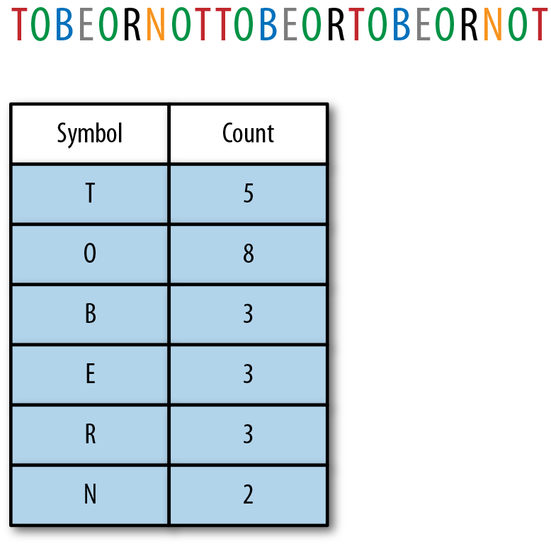
Figure 4-3. A sample string and its histogram, counting the number of occurrences for each character.
Assigning codewords to symbols
Next, sort your histogram by frequency of occurrence (see Figure 4-4), and assign a VLC to each symbol, beginning with the smallest codeword in the VLC set. The end result is that the more frequent the symbol, the smaller its assigned codeword, which results in data compression.
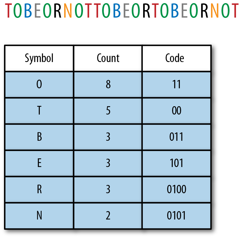
Figure 4-4. After sorting our histogram by symbol count, we can assign codes to symbols. This is often called the “codeword table.” Note that the codewords do not represent standard binary numbers. This is because of the importance of encoding and decoding (which we’re about to discuss).
Encoding
Encoding a stream of symbols with VLCs is very straightforward. You read symbols one by one from the stream. For each symbol read, look up its variable-length code according to the codeword table and emit the bits of that codeword to the output stream. Concatenate the codes to create a single, long bit stream.
After the entire input stream has been processed, attach the symbol-to-codeword table to the head of the output stream, as illustrated in Figure 4-5, so that the decoder can use it to recover the source data.
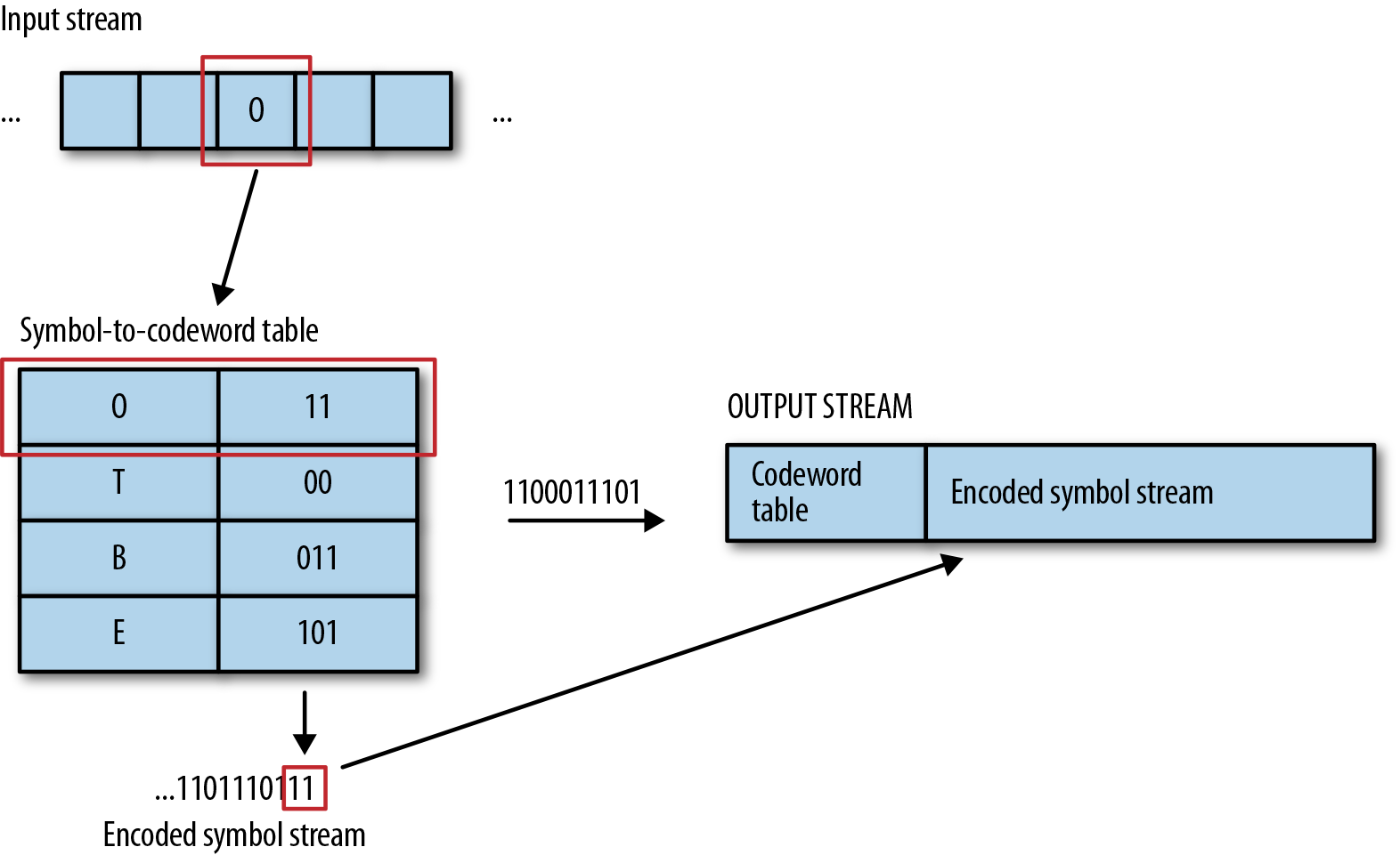
Figure 4-5. Example encoding takes a symbol from the input stream, finds its codeword, and emits the codeword to the output stream. As a final step, the symbol-to-codeword table is prepended to the output data so that the decoder can use it later.
For example, to encode the stream “TOBEORNOT” using the table we just created, the first symbol is a “T,” which emits the codeword 00 to the output stream. “O” follows, outputting 11. This continues, and “TOBEORNOT” ends up as this 24-bit stream: 001101110111010001011100.
Comparing this to the 72-bit source stream (using an even 3 bits per character), we have a savings of roughly 66%.
Decoding
In general, the decoder does the inverse of the encoder. It reads some bits, checks them against the table, finds the correlated symbol, and outputs the symbol to the stream, as shown in Figure 4-6.
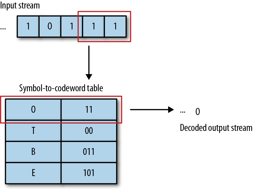
Figure 4-6. Decoding works in reverse. We read in some bits, find the symbol for those bits, and output the symbol.
However, decoding is slightly more complex because of the different lengths of the codewords. Basically, the decoder reads bits one at the time until they match one of the codewords. At that point, it outputs the associated symbol and starts reading for the next codeword.
Let’s look at this with the bit stream we created, 001101110111010001011100, and use the previous table to recover our original string:
-
Read 0.
-
Check the table. There are no single-bit codewords.
-
Read 0. Find the codeword 00. Output T.
-
Read the next bit, which is 1.
-
Read 1 again. Find the codeword 11. Output O.
Now it gets more interesting:
-
Read 0, then read 1. At this point, we have multiple matches in the table. This symbol could be B, R, or N. So we read in a third bit, giving us “011.” Now, we have an exact and unique match with the letter B.
-
In good tradition, decoding the rest is left as an exercise for you to carry out. After you reach the end of the bit stream, you should have recovered the original input string. (Or just refer to Figure 4-7.)

Figure 4-7. Example decoding. We read in each codeword, find the associated symbol in the codeword table, and emit it to the output stream.
Creating VLCs
We want to take a second and point out a small nuance in Morse code. Consider the following Morse encoded message:
•••
Can you figure out what the message is?
Looking back at our table, these three dots appear to be an “S” value.
Take a second look, though. This might also be three E symbols in a row (one dot each).
The ability for an operator to determine which symbol it is has to do with a bit of cheating. See, there are a lot of other things an operator can do to determine what symbol it is. For example, there’s little chance that “eee” would be a valid message in the 1800s, especially if the operator knew its context (CATEEE is not a valid English word, but CATS is).
This extra work that an operator can do to determine the message is not something we can duplicate in the world of compression. We only have 0s and 1s without spaces to work with. As such, Morse code doesn’t work too well as a set of codewords. Instead, we need to find a way to bind 0s and 1s together that lets the decoder uniquely decipher the resulting stream.
The prefix property
So, at any given moment, the decoder needs to be able to take a look at the bits read so far and determine whether they uniquely match the codeword for a symbol, or whether it needs to read another bit. To do this properly, the codewords of the VLC set must take into account two principles:
-
Assign short codes to the most frequent symbols
-
Obey the prefix property
Let’s take a look at how a potential VLC can fall over. Assume the bit stream 0101111 and the following VLC table:
|
Symbol |
Codeword |
|---|---|
|
A |
0 |
|
B |
10 |
|
C |
101 |
|
D |
111 |
Then, the decoding process looks like this:
-
The decoder sees 0, which is unambiguously A. So it outputs A.
-
The decoder sees 1, which can be the beginning of B, C, or D.
-
The decoder reads another 0, which narrows the choice to B or C.
-
The decoder reads 1. This presents an ambiguity. In our bits read, 101, do we have 10 + 1, representing a B plus the beginning of a new symbol B, C, or D?
or
Do we have 101 for a symbol C?
At this point, you can no longer continue with the decoding process, because you’ve lost the ability to determine what type of value is being read in. Your choice of codewords has made it impossible to uniquely distinguish between different symbols, as illustrated in Figure 4-8.
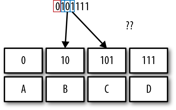
Figure 4-8. Decoding a binary stream with VLCs can be difficult if one code is the prefix of another code.
In comes the VLC prefix property, which dictates:
After a code has been assigned to a symbol, no other code can start with that bit pattern.
In other words, each symbol is unambiguously identifiable by its prefix, which is the only way in which VLCs can work.
Warning
The prefix property is required for a VLC to work properly. This means that VLCs will tend to be larger compared to binary representation.
The general trade-off is that you get a larger code, but you can decode it without knowing anything about symbol size in advance. And because you have some very short codewords for common symbols, VLCs give great compression for symbol streams for which a small number of symbols have very high probability.
A Handful of Example VLCs
In this section, we are going to introduce you to a handful of VLCs that, historically, were commonly used and useful in real life. Choosing the right VLC and assigning the right codes to your symbols is another challenge altogether, as we’ll briefly discuss.
Binary code
We introduced binary code in Chapter 2 and hope you haven’t forgotten everything since then, because binary code is ubiquitous in computing and thus always the end result of compression.
After Peter Elias, it is customary to denote the standard binary representation of the integer n by B(n). This representation is considered the beta or binary code, and it does not satisfy the prefix property. For example, the binary representation of 2 = 102 is also the prefix of 4 =1002.
Now, given a set of integers between 0 and n, we can represent each in 1+floor(log2(n)) bits; that is, we can use a fixed-length representation to get around the prefix issue, as long as we’re provided the value n in advance. In other words, if we know how many numbers we need to represent, we can easily determine how many bits that requires. However, if we don’t know the number of distinct integers in the set in advance, we cannot use a fixed-length representation.
Unary codes
Unary coding represents a positive integer, n, with n - 1 ones followed by a zero. For example, 4 is encoded as 1110.2 The length of a unary code for the integer n, is therefore n bits.
It’s easy to see that the unary code satisfies the prefix property, so you can use it as a variable-length code.
The length of the codewords grows linearly by 1 for increasing numbers n, such that L is always equal to n. In binary, the number of numbers we can represent with each additional bit grows exponentially by 2n. (Remember those 21, 22, etc. columns?)
As such, this code works best when you use it on a data set for which each symbol is twice as probable as the previous. (So, A is two times more frequent than B, which is two times more frequent than C.). Or, if you like math, we can say: in cases for which the input data consists of integers N with exponential probabilities P(n) ~2–n: 1/2, 1/4, 1/8, 1/16, 1/32, and so on.
Here is an example of simple unary encoding with ideal probabilities.
| Number | Code | Ideal probability |
|---|---|---|
|
0 |
|
|
|
1 |
0 |
0.5 |
|
2 |
10 |
0.25 |
|
3 |
110 |
0.125 |
|
4 |
1110 |
0.0625 |
To decode unary encoding, simply read and count value bits from the stream until you hit a delimiter. Add one and output that number.
Elias gamma encoding
Elias gamma encoding is used most commonly for encoding integers whose upper bound cannot be determined beforehand; that is, we don’t know what the largest number is going to be.
The main idea is that instead of encoding the integer directly, we prefix it with an encoded representation of its order of magnitude. This creates a codeword comprising two sections, the largest power of two that fits into the integer plus the remainder, like so:
-
Find the largest integer N, such that 2N < n < 2N + 1 and write n = 2N + L (where L = n - 2N).
-
Encode N in unary.
-
Append L as an N-bit number to this representation. (This is really important because this symmetry is what allows us to decode the string later.)
For example, let’s encode the number n = 12:
-
N is 3, because 23 is 8, and 24 is 16, so that 8 < 12 < 16.
-
L is thus 12 - 8 = 4.
-
N = 3 in unary is 110.
-
L = 4 in binary written with 3 bits is 100.
-
So, our concatenated output is 110100.
To encode a slightly larger number, let’s say 42:
-
N is 5, because 25 is 32, and 32 < 42 < 64.
-
L is thus 42 – 32 = 10.
-
N = 5 in unary is 11110.
-
L = 10 written in 5 bits is 01010.
-
So, our final output is 1111001010.
Elias gamma coding, like simple unary encoding, is ideal for applications for which the probability of n is P(N) = 1/(2n2).
Here is a table with some example Elias gamma codes (note the L part in italics).
| n | 2N + L | Code |
|---|---|---|
|
1 |
20+0 |
0 |
|
2 |
21+0 |
101 |
|
8 |
23+0 |
110000 |
|
12 |
23+4 |
110100 |
|
42 |
25+10 |
1111001010 |
Decoding Elias gamma is also straightforward:
-
Let’s take the number 12, which we encoded as 110100.
-
Read values until we get to the delimiter: 1, 1, 0. This gives us N = 3.
-
Read 3 more bits 1,0,0 and convert from binary, which gives us L = 4.
-
Combine 2N + L = 23 + 4 = 12.
Elias delta coding
Elias delta is another variation on the same theme. In this code, Elias prepends the length in binary, making this code slightly more complex.
It works like this:
-
Write your original number, n, in binary.
-
Count the bits in binary n, and convert that count to binary, which gives us C.
-
Remove the leftmost bit of binary n, which is always one and thus can be implied.
-
Prepend the count C, in binary, to what is left of n after its leftmost bit has been removed.
-
Subtract 1 from the length of the count of C and prepend that number of zeros to the code.
For example, let’s again encode the number n = 12:
-
Write n = 12 in binary, which is n = 1100.
-
The binary version of 12 has 4 bits, and converted to binary, that is C = 100.
-
Remove the leftmost bit of n = 1100, leaving you with 100.
-
Prepend C = 100 to what’s left of n, which is 100, giving you 100100.
-
Subtract 1 from the length of C, 3 – 1 = 2, and prepend that many zeros to the code, giving you a final encoding of 00100100 for 12.
Elias delta is ideal for data for which n occurs with a probability of 1/[2n(log2(2n))2].
Here is a table with some example Elias delta codings:
| n in decimal | 2N + L | Code |
|---|---|---|
|
1 |
20+0 |
0 |
|
2 |
21+0 |
0100 |
|
8 |
23+0 |
00100000 |
|
12 |
23+4 |
00100100 |
|
18 |
24+2 |
001010010 |
|
314 |
28 + 58 |
000100100111010 |
To decode Elias delta, do the following:
-
Read and count 0s until you hit 1.
-
Add 1 to the count of zeros, which gives you the length of C.
-
Read length of C many more bits, which gives you C.
-
Read C - 1 more bits, prepend 1, and convert to decimal.
Using our handy number 00100100:
-
Read and count 0s until you hit 1, which is 2 zeros.
-
Add 1, yielding a length of C = 3.
-
Read 3 more bits, giving you C = 100 = 4
-
Read 4 - 1 more bits, which is 100, and prepend 1, yielding 1100, which is 12.
If you don’t believe this works, encode and decode the provided value 314 as an example.
And so many more!
So, now that you have worked your way through a couple of the simpler variable-length encoding algorithms, and get the gist of it, we need to tell you that there are literally hundreds of unique VLCs that have been created over the past 40 years, and we can’t cover every single one of them in this book.
Finding the Right Code for Your Data Set
The biggest difference between the codes we introduced is that each of these code sets behaves differently, given their expectation of the frequency distribution of the symbols.
So, when choosing a VLC code for your data set, you first must consider its size and range, and calculate the probabilities of its symbols. If you don’t do that, encoding your data might end up not only not compressing it—you might actually end up with a much larger stream.
To get a sense of how different this is, per code, the following table shows that for a given symbol, and a probability matching each of the encodings, how many bits per symbol are needed.
| Number of symbols |
Elias gamma Number of bits needed for a probability distribution matching each encoding 1 / (2n2) |
Elias delta 1 / [2n(log2(2n))2] |
Elias omegaa Largest encoded value is not known ahead of time, and small values are much more frequent than large values |
|---|---|---|---|
|
1 |
1 |
1 |
2 |
|
2 |
3 |
4 |
3 |
|
3 |
3 |
4 |
4 |
|
8–15 |
7 |
8 |
6–7 |
|
64–88 |
13 |
11 |
10 |
|
100 |
13 |
11 |
11 |
|
1000 |
19 |
16 |
16 |
a More information on Elias omega. | |||
What You Need to Remember
VLCs assign bits to codewords based upon the expected frequency of occurrence of a value. As such, each VLC is built with its own expectation as to how the probabilities of symbols are distributed in the data set. The trick, then, is finding the right VLC, the one that’s built with a statistical model that matches your data. If you diverge from that, you’ll end up with a bloated data stream.
For the first 15 or so years of information theory, compression technology was completely limited to VLCs. Basically, to compress a data set, an engineer would need to find the right code to match their set, and use it appropriately.
Thankfully, this isn’t how things are done anymore.
In the next chapter, we are going to talk about how you can generate your very own VLCs using nothing but sticky notes and a pen.
2 Note, you could flip the bits here, if you wanted, and make it 0001. The basic idea is that some bit is used as the value, and the other bit is used as the delimiter.
3 L. Thiel and H. Heaps, “Program Design for Retrospective Searches on Large Data Bases,” Information Storage and Retrieval 1972; 8(1):1–20
Get Understanding Compression now with the O’Reilly learning platform.
O’Reilly members experience books, live events, courses curated by job role, and more from O’Reilly and nearly 200 top publishers.

