The R Book

Three-Dimensional Plots

When there are two continuous explanatory variables, it is often useful to plot the response as a contour map. In this example, the biomass of one plant species (the response variable) is plotted against soil pH and total community biomass. The species is a grass called Festuca rubra that peaks in abundance in communities of intermediate total biomass:

data < -read.table("c: \\ temp \\ pgr.txt",header=T)
attach(data)
names(data)

[1] "FR" "hay" "pH"

You need the library called akima in order to implement bivariate interpolation onto a grid for irregularly spaced input data like these, using the function interp:

install.packages("akima")
library(akima)

The two explanatory variables are presented first (hay and pH in this case), with the response variable (the ‘height’ of the topography), which is FR in this case, third:

zz < -interp(hay,pH,FR)

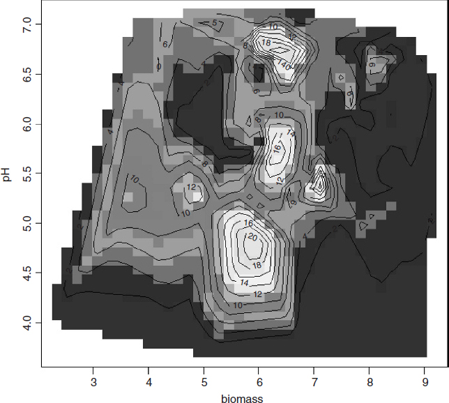
The list called zz can now be used in any of the four functions contour, filled.contour, image or persp. We start by using contour and image together. Rather than the red and yellows of heat.colors we choose the cooler blues and greens of topo.colors:

image(zz,col = topo.colors(12),xlab="biomass",ylab="pH")
contour(zz,add=T)

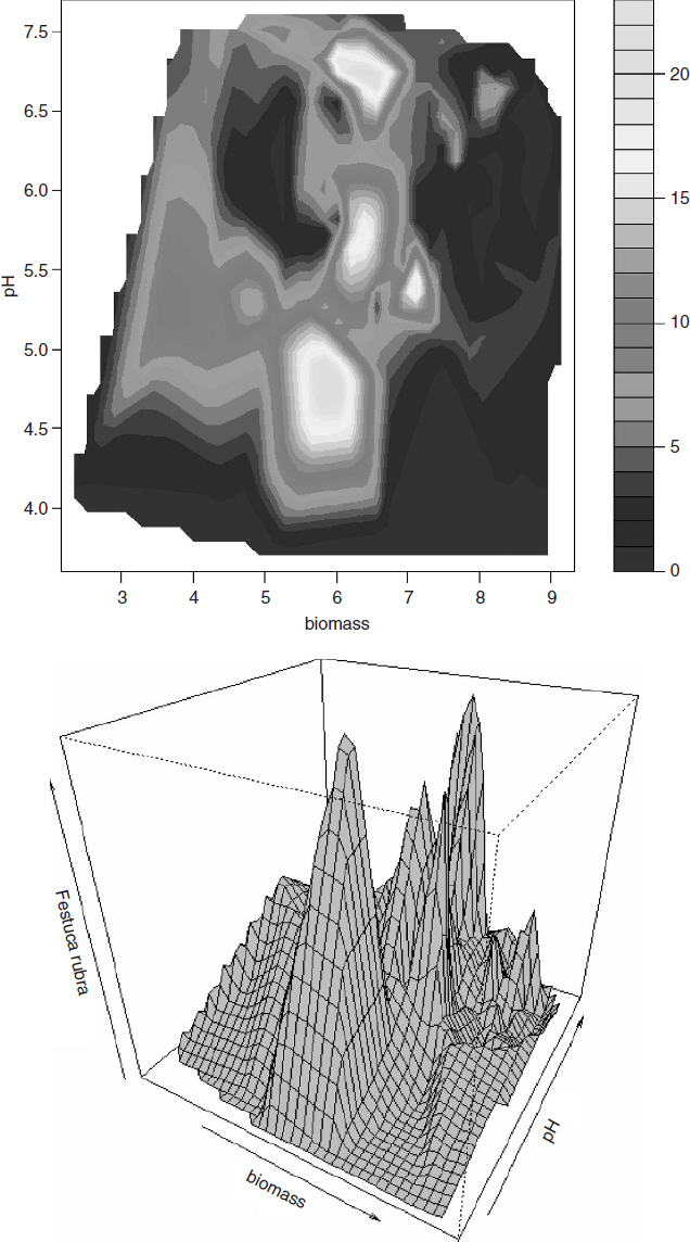
Alternatively, you can use the filled.contour function,

filled.contour(zz,col = topo.colors(24),xlab="biomass",ylab="pH") ...