Parametric analysis
The following example concerns survivorship of two cohorts of seedlings. All the seedlings died eventually, so there is no censoring in this case. There are two questions:
- Was survivorship different in the two cohorts?
- Was survivorship affected by the size of the canopy gap in which germination occurred?
Here are the data:
seedlings<-read.table("c:\\temp\\seedlings.txt",header=T)
attach(seedlings)
names(seedlings)

[1]  "cohort"  "death"  "gapsize"
We need to load the survival library:
library(survival)
We begin by creating a variable called status to indicate which of the data are censored:
status<-1*(death>0)
There are no cases of censoring in this example, so all of the values of status are equal to 1.
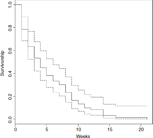
The fundamental object in survival analysis is Surv(death,status), the Kaplan–Meier survivorship object. We can plot it out using survfit with plot like this:
plot(survfit(Surv(death,status)),ylab="Survivorship",xlab="Weeks")
This shows the overall survivorship curve with the confidence intervals. All the seedlings were dead by week 21. Were there any differences in survival between the two cohorts?
model<-survfit(Surv(death,status)~cohort)
summary(model)

Call: survfit(formula = Surv(death, status) ~ cohort)

              cohort=October
time n.risk n.event survival std.err lower 95% CI upper 95% CI 1 30 7 0.7667 0.0772 0.62932 0.934 2 23 3 0.6667 0.0861 0.51763 0.859 ...
Get The R Book now with the O’Reilly learning platform.
O’Reilly members experience books, live events, courses curated by job role, and more from O’Reilly and nearly 200 top publishers.

