Background
Since everything dies eventually, it is often not possible to analyse the results of survival experiments in terms of the proportion that were killed (as we did in Chapter 16); in due course, they all die. Look at the following figure:
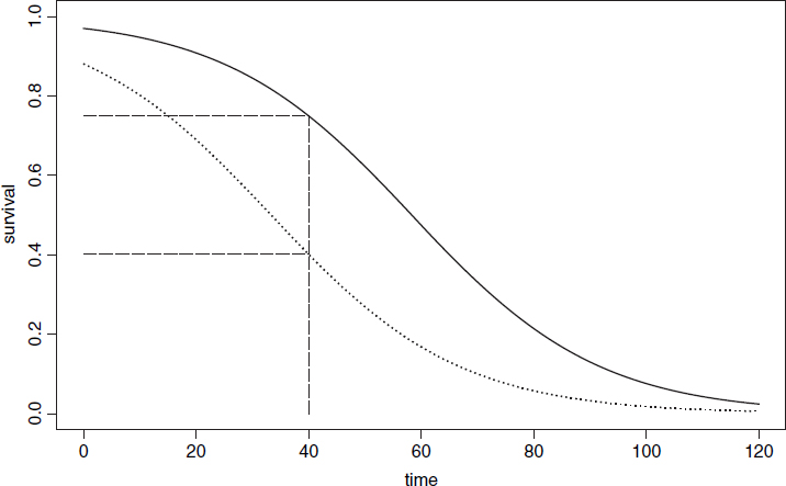
It is clear that the two treatments caused different patterns of mortality, but both start out with 100% survival and both end up with zero. We could pick some arbitrary point in the middle of the distribution at which to compare the percentage survival (say at time = 40), but this may be difficult in practice, because one or both of the treatments might have few observations at the same location. Also, the choice of when to measure the difference is entirely subjective and hence open to bias. It is much better to use R's powerful facilities for the analysis of survival data than it is to pick an arbitrary time at which to compare two proportions.
Demographers, actuaries and ecologists use three interchangeable concepts when dealing with data on the timing of death: survivorship, age at death and instantaneous risk of death. There are three broad patterns of survivorship: Type I, where most of the mortality occurs late in life (e.g. humans); Type II, where mortality occurs at a roughly constant rate throughout life; and Type III, where most of the mortality occurs early in life (e.g. salmonid fishes). On a log scale, the numbers surviving ...
Get The R Book now with the O’Reilly learning platform.
O’Reilly members experience books, live events, courses curated by job role, and more from O’Reilly and nearly 200 top publishers.

