The R Book

Time series modelling on the Canadian lynx data

Records of the number of skins of predators (lynx) and prey (snowshoe hares) returned by trappers were collected over many years by the Hudson's Bay Company. The lynx numbers are shown on p. 717 and exhibit a clear 10-year cycle. We begin by plotting the autocorrelation and partial autocorrelation functions:

par(mfrow=c(1,2))
acf(Lynx,main="")
acf(Lynx,type="p",main="")

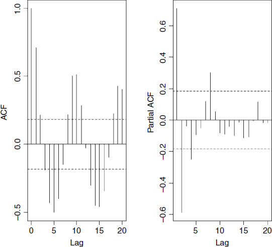
The population is very clearly cyclic, with a period of 10 years. The dynamics appear to be driven by strong, negative density dependence (a partial autocorrelation of −0.588) at lag 2. There are other significant partials at lag 1 and lag 8 (positive) and lag 4 (negative). Of course you cannot infer the mechanism by observing the dynamics, but the lags associated with significant negative and positive feedbacks are extremely interesting and highly suggestive. The main prey species of the lynx is the snowshoe hare and the negative feedback at lag 2 may reflect the timescale of this predator–prey interaction. The hares are known to cause medium-term induced reductions in the quality of their food plants as a result of heavy browsing pressure when the hares at high density, and this could map through to lynx populations with lag 4.

The order vector specifies the non-seasonal part of the ARIMA model: the three components (p, d, q) are the AR order, the degree of differencing, ...