Simulated Time Series
To see how the correlation structure of an AR(1) depends on the value of α, we can simulate the process over, say, 250 time periods using different values of α. We generate the white noise Zt using the random number generator rnorm(n,0,s) which gives n random numbers with a mean of 0 and a standard deviation of s. To simulate the time series we evaluate
![]()
multiplying last year's population by α then adding the relevant random number from Zt.
We begin with the special case of α = 0 so Yt = Zt and the process is pure white noise:
Y<-rnorm(250,0,2)
par(mfrow=c(1,2))
plot.ts(Y)
acf(Y)
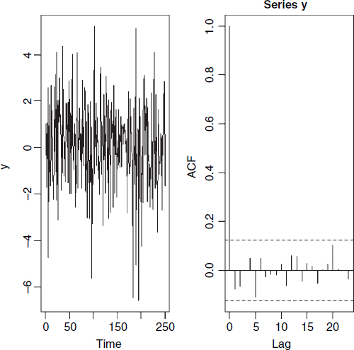
The time series is bound to be stationary because each value of Z is independent of the value before it. The correlation at lag 0 is 1 (of course), but there is absolutely no hint of any correlations at higher lags.
To generate the time series for non-zero values of α we need to use recursion: this year's population is last years population times α plus the white noise. We begin with a negative value of α = −0.5. First we generate all the noise values (by definition, these don't depend on population size):
Z<-rnorm(250,0,2)
Now the initial population at time 0 is set to 0 (remember that the population is stationary, so we can think of the Y values as departures from the long-term ...
Get The R Book now with the O’Reilly learning platform.
O’Reilly members experience books, live events, courses curated by job role, and more from O’Reilly and nearly 200 top publishers.

