Multiple Time Series
When we have two or more time series measured over the same period, the question naturally arises as to whether or not the ups and downs of the different series are correlated. It may be that we suspect that change in one of the variables causes changes in the other (e.g. changes in the number of predators may cause changes in the number of prey, because more predators means more prey eaten). We need to be careful, of course, because it will not always be obvious which way round the causal relationship might work (e.g. predator numbers may go up because prey numbers are higher; ecologists call this a numerical response). Suppose we have the following sets of counts:
twoseries<-read.table("c:\\temp\\twoseries.txt",header=T)
attach(twoseries)
names(twoseries)

[1] "x" "y"
We start by inspecting the two time series one above the other:
plot.ts(cbind(x,y),main="")
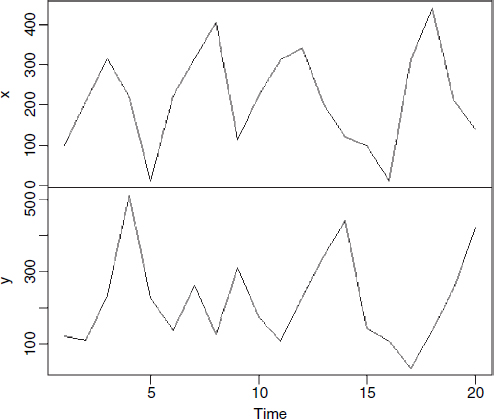
There is some evidence of periodicity (at least in x) and it looks as if y lags behind x by roughly 2 periods (sometimes 1). Now let's carry out straightforward analyses on each time series separately:
par(mfrow=c(1,2))
acf(x,type="p")
acf(y,type="p")
As we suspected, the evidence for periodicity is stronger in x than in y: the partial autocorrelation is significant and negative at lag 2 for x, but none of the partial autocorrelations are significant for y.
To look at the cross-correlation between ...
Get The R Book now with the O’Reilly learning platform.
O’Reilly members experience books, live events, courses curated by job role, and more from O’Reilly and nearly 200 top publishers.

