Spectral Analysis
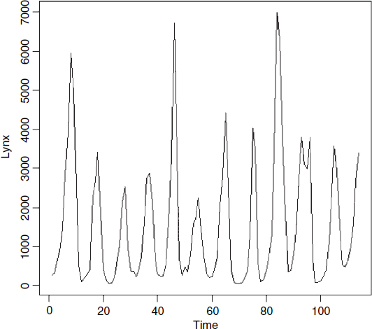
There is an alternative approach to time series analysis, which is based on the analysis of frequencies rather than fluctuations of numbers. Frequency is the reciprocal of cycle period. Ten-year cycles would have a frequency 0.1 per year. Here are the famous Canadian lynx data:
numbers<-read.table("c:\\temp\\lynx.txt",header=T)
attach(numbers)
names(numbers)

[1] "Lynx"

plot.ts(Lynx)
The fundamental tool of spectral analysis is the periodogram. This is based on the squared correlation between the time series and sine/cosine waves of frequency ω, and conveys exactly the same information as the autocovariance function. It may (or may not) make the information easier to interpret. Using the function is straightforward; we employ the spectrum function like this:
spectrum(Lynx)
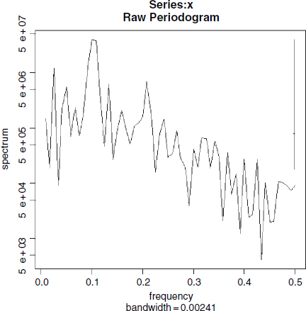
The plot is on a log scale, in units of decibels, and the sub-title on the x axis shows the bandwidth, while the 95% confidence interval in decibels is shown by the vertical bar in the top right-hand corner. The figure is interpreted as showing strong cycles with a frequency of about 0.1, where the maximum value of spectrum occurs. That is to say, it indicates cycles with a period of 1/0.1 = 10 years. There is a hint of longer period cycles (the local peak at frequency 0.033 would produce cycles ...
Get The R Book now with the O’Reilly learning platform.
O’Reilly members experience books, live events, courses curated by job role, and more from O’Reilly and nearly 200 top publishers.

