Seasonal Data
Many time series applications involve data that exhibit seasonal cycles. The commonest applications involve weather data: here are daily maximum and minimum temperatures from Silwood Park in south-east England over the period 1987–2005 inclusive:
weather<-read.table("c:\\temp\\SilwoodWeather.txt",header=T)
attach(weather)
names(weather)

[1]   "upper"  "lower" "rain" "month" "yr"

plot(upper,type="l")
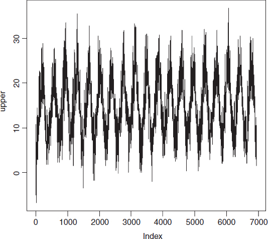
The seasonal pattern of temperature change over the 19-year period is clear, but there is no clear trend (e.g. warming, see p. 715). Note that the x axis is labelled by the day number of the time series (Index).
We start by modelling the seasonal component. The simplest models for cycles are scaled so that a complete annual cycle is of length 1.0 (rather than 365 days). Our series consists of 6940 days over a 19-year span, so we write:
length(upper)

[1] 6940

index<-1:6940
6940/19

[1] 365.2632

time<-index/365.2632
The equation for the seasonal cycle is this:
![]()
This is a linear model, so we can estimate its three parameters very simply:
model<-lm(upper~sin(time*2*pi)+cos(time*2*pi))
To investigate the fit of this model we need to plot the scattergraph using very small symbols (otherwise the fitted line will be completely obscured). The smallest useful plotting symbol is the ...
Get The R Book now with the O’Reilly learning platform.
O’Reilly members experience books, live events, courses curated by job role, and more from O’Reilly and nearly 200 top publishers.

