Self-starting four-parameter logistic
This model allows a lower asymptote (the fourth parameter) as well as an upper:
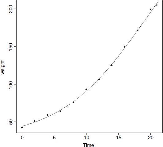
data<-read.table("c:\\temp\\chicks.txt",header=T)
attach(data)
names(data)

[1] "weight"  "Time"

model <- nls(weight~SSfpl(Time, a, b, c, d))
xv<-seq(0,22,.2)
yv<-predict(model,list(Time=xv))
plot(weight~Time,pch=16)
lines(xv,yv)

summary(model)
Formula: weight~SSfpl(Time, a, b, c, d)

Parameters:
   Estimate  Std. Error  t value    Pr(>|t|)
a    27.453       6.601    4.159    0.003169  **
b   348.971      57.899    6.027    0.000314  ***
c    19.391       2.194    8.836    2.12e-05  ***
d     6.673       1.002    6.662    0.000159  ***

Residual standard error: 2.351 on 8 degrees of freedom
The four-parameter logistic is given by
![]()
This is the same formula as we used in Chapter 7, but note that C above is 1/c on p. 203. A is the horizontal asymptote on the left (for low values of x), B is the horizontal asymptote on the right (for large values of x), D is the value of x at the point of inflection of the curve (represented by xmid in our model for the chicks data), and C is a numeric scale parameter on the x axis (represented by scal). The parameterized model would be written like this:
![]()
Self-starting Weibull growth function
R's parameterization ...
Get The R Book now with the O’Reilly learning platform.
O’Reilly members experience books, live events, courses curated by job role, and more from O’Reilly and nearly 200 top publishers.

