Regression in Mixed-Effects Models
The next example involves a regression of plant size against local point measurements of soil nitrogen (N) at five places within each of 24 farms. It is expected that plant size and soil nitrogen will be positively correlated. There is only one measurement of plant size and soil nitrogen at any given point (i.e. there is no temporal pseudoreplication; cf. p. 629):
yields<-read.table("c:\\temp\\farms.txt",header=T)
attach(yields)
names(yields)

[1]  "N"  "size"  "farm"
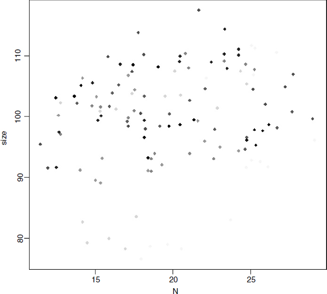
Here are the data in aggregate, with different plotting colours for each farm:
plot(N,size,pch=16,col=farm)
The most obvious pattern is that there is substantial variation in mean values of both soil nitrogen and plant size across the farms: the minimum (yellow) fields have a mean y value of less than 80, while the maximum (red) fields have a mean y value above 110.
The key distinction to understand is between fitting lots of linear regression models (one for each farm) and fitting one mixed-effects model, taking account of the differences between farms in terms of their contribution to the variance in response as measured by a standard deviation in intercept and a standard deviation in slope. We investigate these differences by contrasting the two fitting functions, lmList and lme. We begin by fitting 24 separate linear models, one for each farm:
linear.models<-lmList(size~N|farm,yields) ...Get The R Book now with the O’Reilly learning platform.
O’Reilly members experience books, live events, courses curated by job role, and more from O’Reilly and nearly 200 top publishers.

