Generalized Additive Models
This dataframe contains measurements of radiation, temperature, wind speed and ozone concentration. We want to model ozone concentration as a function of the three continuous explanatory variables using non-parametric smoothers rather than specified nonlinear functions (the parametric multiple regression analysis is on p. 434):
ozone.data<-read.table("c:\\temp\\ozone.data.txt",header=T)
attach(ozone.data)
names(ozone.data)
[1] "rad" "temp" "wind" "ozone"
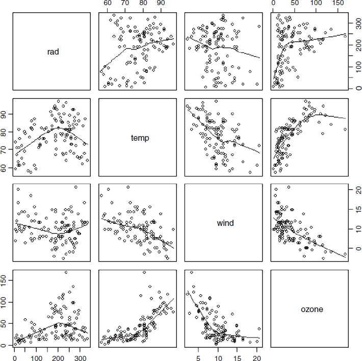
For data inspection we use pairs with a non-parametric smoother, lowess:
pairs(ozone.data, panel=function(x,y) { points(x,y); lines(lowess(x,y))} )
Now fit all three explanatory variables using the non-parametric smoother s():
model<-gam(ozone~s(rad)+s(temp)+s(wind))
summary(model)

Family: gaussian
Link function: identity

Formula:
ozone ~ s(rad) + s(temp) + s(wind)
Parametric coefficients:

              Estimate   Std. Error  t value  Pr( > |t|)
(Intercept)      42.10         1.66    25.36     < 2e-16    ***
Approximate significance of smooth terms:
             edf  Est.rank        F    p-value
s(rad)     2.763     6.000    2.830     0.0138    *
s(temp)    3.841     8.000    8.080   2.27e-08    ***
s(wind)    2.918     6.000    8.973   7.62e-08    ***
R-sq.(adj) = 0.724 Deviance explained = 74.8%
GCV score = 338 Scale est. = 305.96 n = 111
Note that the intercept is estimated as a parametric coefficient (upper table) and the three explanatory variables are fitted as smooth terms. All three are significant, ...
Get The R Book now with the O’Reilly learning platform.
O’Reilly members experience books, live events, courses curated by job role, and more from O’Reilly and nearly 200 top publishers.

