The R Book

Model checking in R

The data we examine in this section are on the decay of a biodegradable plastic in soil: the response, y, is the mass of plastic remaining and the explanatory variable, x, is duration of burial:

Decay<-read.table("c:\\temp\\Decay.txt",header=T)
attach(Decay)
names(Decay)

[1] "time" "amount"

For the purposes of illustration we shall fit a linear regression to these data and then use model-checking plots to investigate the adequacy of that model:

model<-lm(amount ~ time)

The basic model checking could not be simpler:

plot(model)

This one command produces a series of graphs, spread over four pages. The first two graphs are the most important. First, you get a plot of the residuals against the fitted values (left plot) which shows very pronounced curvature; most of the residuals for intermediate fitted values are negative, and the positive residuals are concentrated at the smallest and largest fitted values. Remember, this plot should look like the sky at night, with no pattern of any sort. This suggests systematic inadequacy in the structure of the model. Perhaps the relationship between y and x is non-linear rather than linear as we assumed here? Second, you get a QQ plot (p. 341) which indicates pronounced non-normality in the residuals (the line should be straight, not banana-shaped as here).

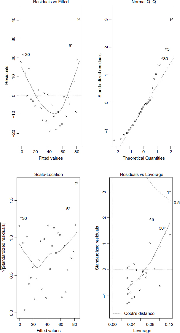
The third graph is like a positive-valued version of the first ...