Continuous Probability Distributions
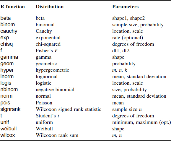
R has a wide range of built-in probability distributions, for each of which four functions are available: the probability density function (which has a d prefix); the cumulative probability (p); the quantiles of the distribution (q); and random numbers generated from the distribution (r). Each letter can be prefixed to the R function names in Table 7.1 (e.g. dbeta).
Table 7.1. The probability distributions supported by R. The meanings of the parameters are explained in the text.
The cumulative probability function is a straightforward notion: it is an S-shaped curve showing, for any value of x, the probability of obtaining a sample value that is less than or equal to x. Here is what it looks like for the normal distribution:
curve(pnorm(x),-3,3)
arrows(-1,0,-1,pnorm(-1),col="red")
arrows(-1,pnorm(-1),-3,pnorm(-1),col="green")
The value of x(−1) leads up to the cumulative probability (red arrow) and the probability associated with obtaining a value of this size (−1) or smaller is on the y axis (green arrow). The value on the y axis is 0.158 655 3:
pnorm(-1)

[1]  0.1586553
The probability densityis the slope of this curve (its ‘derivative’). You can see at once that the slope is never negative. The slope starts out very shallow up to about x = −2, increases up to a peak (at x = 0 in this example) then gets shallower, and becomes very small indeed ...
Get The R Book now with the O’Reilly learning platform.
O’Reilly members experience books, live events, courses curated by job role, and more from O’Reilly and nearly 200 top publishers.

