CHAPTER 2
Preliminary Mathematical Tools
2.1. PROBABILITY DISTRIBUTIONS
A review of discrete and continuous probability distributions is an appropriate first step to outline the mathematics of derivatives.
If pi (or P(x)dx) represents the probability of an “occurrence” at discrete coordinate xi (or in range x → x + dx), then we can model a person’s ability to throw darts, say, by the probability distribution of the results of their throwing darts at a board, aiming to hit only the bull’s-eye. The distribution would likely be angularly symmetric and would peak around the bull’s-eye and fall off farther away. This means that the thrower has a good enough eye that his throws usually come close to the bull’s-eye. We might even measure his skill level by trying to measure the distribution.
Presumably, the average result of many throws
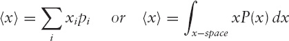
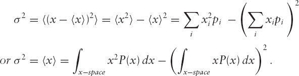
will be close to the bull’s-eye, and would get closer and closer as more and more throws are observed and so contains little or no information about the thrower’s skill level. On the other hand, the width of the distribution (or radius of the central lump of distribution of throws) can be measured as the standard deviation σ where
EXPECTATION VALUES AND AVERAGES
The average of N values x1, x2, . . ., xN, is often written as
Now if the N values are selected ...
Get The Mathematics of Derivatives: Tools for Designing Numerical Algorithms now with the O’Reilly learning platform.
O’Reilly members experience books, live events, courses curated by job role, and more from O’Reilly and nearly 200 top publishers.

