The Mathematics of Derivatives: Tools for Designing Numerical Algorithms

APPENDIX A

Central Limit Theorem-Plausibility Argument

If a path begins at a point x₀ then the initial distribution over x is the Dirac delta distribution, which means merely that the path has probability 1 of being located exactly at the starting point, expressed as

p(x; t = 0) = δ(x − x₀).

Then use a square shock, meaning that the distribution is convoluted with a square of width 2α and height 1/(2α),

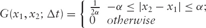
and the new distribution is then a square. Then convolute again and the new distribution is a triangle,

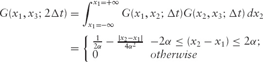
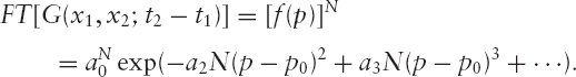
and so on. Now, in more general terms, let the shock be some function f(x), not necessarily a square. Fourier transform the function to get f(p), and expand it as follows:

f(p) = a₀ exp(−a₂(p − p₀)² + a₃(p − p₀)³ + · · ·)

about its maximum, at p₀. This expansion is meaningful as long as the derivative of f(p) is zero and continuous at p₀ and the second derivative of f(p) is continuous and negative (i.e., a₂ > 0). Then take the N-th power of this, to get the Fourier transform of the operator that gives us the N-step distribution:

Now the argument is that because the first term looks like the Fourier transform of a Gaussian of standard deviation

and for a particular standard deviation, ...