Chapter 4. Maneuvering
Thinking SQL Statements
There is only one principle of war, and that’s this. Hit the other fellow, as quickly as you can, as hard as you can, where it hurts him most, when he ain’t lookin’.
—Field Marshal Sir William Slim (1891-1970) quoting an anonymous Sergeant-Major
In this chapter, we are going to take a close look at the SQL query and examine how its construct can vary according to the tactical demands of particular situations. This will involve examining complex queries and reviewing how they can be decomposed into a succession of smaller components, all interdependent, and all contributing to a final, complete query.
The Nature of SQL
Before we begin examining query constructs in detail, we need to review some of the general characteristics of SQL itself: how it relates to the database engine and the associated optimizer, and what may limit the efficiency of the optimizer.
SQL and Databases
Relational databases owe their existence to pioneering work by E.F. Codd on the relational theory. From the outset, Codd’s work provided a very strong mathematical basis to what had so far been a mostly empirical discipline. To make an analogy, for thousands of years mankind has built bridges to span rivers, but frequently these structures were grossly overengineered simply because the master builders of the time didn’t fully understand the true relationships between the materials they used to build their bridges, and the consequent strengths of these bridges. Once the science of civil engineering developed a solid theoretical knowledge of material strengths, bridges of a far greater sophistication and safety began to emerge, demonstrating the full exploitation of the various construction materials being used. Indeed, the extraordinary dimensions of some modern bridges reflect the similarly huge increase in the data volumes that modern DBMS software is able to address. Relational theory has done for databases what civil engineering has done for bridges.
It is very common to find confusion between the SQL language, databases, and the relational model. The function of a database is primarily to store data according to a model of the part of the real world from which that data has been obtained. Accordingly, a database must provide a solid infrastructure that will allow multiple users to make use of that same data, without, at any time, prejudicing the integrity of that data when they change it. This will require the database to handle contention between users and, in the extreme case, to keep the data consistent if the machine were to fail in mid-transaction. The database must also perform many other functions outside the scope of this book.
As its name says, Structured Query Language, or SQL for short, is nothing other than a language, though admittedly with a very tight coupling to databases. Equating the SQL language with relational databases —or even worse with the relational theory—is as misguided as assuming that familiarity with a spreadsheet program or a word processor is indicative of having mastered “information technology.” In fact, some products that are not databases support SQL,[*] and before becoming a standard SQL had to compete against other languages such as RDO or QUEL, which were considered by many theorists to be superior to SQL.
Whenever you have to solve what I shall generically call an SQL problem, you must realize that there are two components in action: the SQL expression of the query and the database optimizer. These two components interact within three distinct zones, as shown in Figure 4-1. At the center lies the relational theory , where mathematicians freely roam. If we simplify excessively, we can say that (amongst other useful things) the theory informs us that we can retrieve data that satisfies some criteria by using a handful of relational operators, and that these operators will allow us to answer basically any question. Most importantly, because the relational theory is so firmly grounded in mathematics, we can be totally confident that relational expressions can be written in different ways and yet return the same result. In exactly the same way, arithmetic teaches us that 246/369 is exactly the same as 2/3.
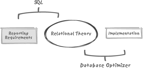
However, despite the crucial theoretical importance of relational theory, there are aspects of great practical relevance that the relational theory has nothing to say about. These fall into an area I call “reporting requirements .” The most obvious example in this area is the ordering of result sets. Relational theory is concerned only with the retrieval of a correct data set, as defined by a query. As we are practitioners and not theorists, for us the relational phase consists in correctly identifying the rows that will belong to our final result set. The matter of how some attributes (columns) of one row relate to similar attributes in another row doesn’t belong to this phase, and yet this is what ordering is all about. Further, relational theory has nothing to say about the numerous statistical functions (such as percentiles and the like) that often appear in various dialects of the SQL language. The relational theory operates on set, and knows nothing of the imposition of ordering on these sets. Despite the fact that there are many mathematical theories built around ordering, none have any relevance to the relational theory.
At this stage I must point out that what distinguishes
relational operations from what I have called reporting
requirements is that relational operations apply to
mathematical sets of theoretically infinite extent. Irrespective of
whether we are operating on tables of 10, one million, or one billion
rows, we can apply any filtering criterion in an identical fashion.
Once again, we are concerned only with identifying and returning the
data that matches our criteria. Here, we are in the environment where
the relational theory is fully applicable. Now, when we want to order
rows (or perform an operation such as group
by that most people would consider a relational operation)
we are no longer working on a potentially infinite data set, but on a
necessarily finite set. The consequent data set thus ceases to be a
relation in the mathematical sense of the word. We are outside the
bounds of the relational theory. Of course, this doesn’t mean that we
cannot still do clever and useful things against this data using
SQL.
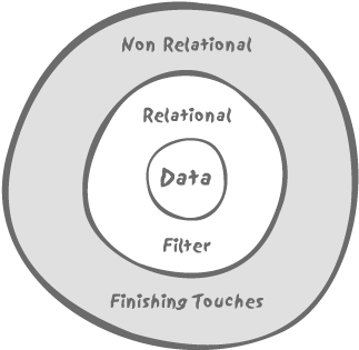
So we may, as a first approximation, represent an SQL query as a double-layered operation as shown in Figure 4-2; first, a relational core identifying the set of data we are going to operate on, second, a non-relational layer which works on this now finite set to give the polishing touch and produce the final result that the user expects.
Despite Figure 4-2’s
appealingly simple representation of the place of SQL within the data
environment, an SQL query will in most cases be considerably more
complex than Figure 4-2
may suggest; Figure 4-2
only represents the overall pattern. The relational filter may be a
generic name for several independent filters combined, for instance,
through a union construct or by the
means of subqueries, and the complexity of some SQL constructs can be
considerable. I shall come back to the topic of SQL code a little
later. But first I must talk about the relationship between the
physical implementation of data and the database optimizer.
SQL and the Optimizer
An SQL engine that receives a query to process will have to use the optimizer to find out how to execute that query in the most efficient way possible. Here the relational theory strikes again, because that theory informs the optimizer of transformations that are valid equivalents of the semantically correct query initially provided by the developer—even if that original query was clumsily written.
Optimization is when the physical implementation of data comes into play. Depending on the existence of indexes and their usability in relation to a query, some transformations may result in much faster execution than other semantically equivalent transformations. Various storage models that I introduce in Chapter 5 may also make one particular way to execute a query irresistibly attractive. The optimizer examines the disposition of the indexes that are available, the physical layout of data, how much memory is available, and how many processors are available to be applied to the task of executing the query. The optimizer will also take into account information concerning the volume of the various tables and indexes that may be involved, directly or indirectly, through views used by the query. By weighing the alternatives that theory says are valid equivalents against the possibilities allowed by the implementation of the database, the optimizer will generate what is, hopefully, the best execution plan for the query.
However, the key point to remember is that, although the optimizer may not always be totally weaponless in the non-relational layer of an SQL query, it is mainly in the relational core that it will be able to deploy its full power—precisely because of the mathematical underpinnings of the relational theory. The transformation from one SQL query to another raises an important point: it reminds us that SQL is supposed to be a declarative language . In other words, one should use SQL to express what is required, rather than how that requirement is to be met. Going from what to how, should, in theory, be the work of the optimizer.
You saw in Chapters 1 and 2 that SQL queries are only some of the variables in the equation; but even at the tactical query level, a poorly written query may prevent the optimizer from working efficiently. Remember, the mathematical basis of the relational theory provides an unassailable logic to the proceedings. Therefore, part of the art of SQL is to minimize the thickness, so to speak, of the non-relational layer—outside this layer, there is not much that the optimizer can safely do that guarantees returning exactly the same rows as the original query.
Another part of the art of SQL is that when performing non-relational operations—loosely defined as operations for which the whole (at least at this stage) resulting dataset is known—we must be extremely careful to operate on only the data that is strictly required to answer the original question, and nothing more. Somehow, a finite data set, as opposed to the current row, has to be stored somewhere, and storing anything in temporary storage (memory or disk) requires significant overhead due to byte-pushing. This overhead may dramatically increase as the result set data volumes themselves increase, particularly if main memory becomes unavailable. A shortage of main memory would initiate the high-resource activity of swapping to disk, with all its attendant overheads. Moreover, always remember that indexes refer to disk addresses, not temporary storage—as soon as the data is in temporary storage, we must wave farewell to most fast access methods (with the possible exception of hashing).
Some SQL dialects mislead users into believing that they are
still in the relational world when they have long since left it. Take
as a simple example the query “Who are the five top earners among
employees who are not executives?”—a reasonable real-life question,
although one that includes a distinctly non-relational twist.
Identifying employees who are not executives is the relational part of
the query, from which we obtain a finite set of employees that we can
order. Several SQL dialects allow one to limit the number of rows
returned by adding a special clause to the select statement. It is
then fairly obvious that both the ordering and
the limitation criteria are outside the
relational layer. However, other dialects, the Oracle version figuring
prominently here, use other mechanisms. What Oracle has is a dummy
column named rownum that applies a
sequential numbering to the rows in the order in which they are
returned—which means the numbering is applied during the relational
phase. If we write something such as:
select empname, salary
from employees
where status != 'EXECUTIVE'
and rownum <= 5
order by salary descwe get an incorrect result, at least in the sense that we are not getting the top five most highly paid nonexecutives, as the query might suggest at first glance. Instead, we get back the first five nonexecutives found—they could be the five lowest paid!—ordered in descending order of salary. (This query illustrates a well-known trap among Oracle practitioners, who have all been burnt at least once.)
Let’s just be very clear about what is happening with the
preceding query. The relational component of the query simply retrieves the first five rows
(attributes empname and salary only) from the table employees where the employee is not an
executive in a totally unpredictable order.
Remember that relational theory tells us that a relation (and
therefore the table that represents it) is not defined in any way by
the order in which tuples (and therefore the rows in that table) are
either stored or retrieved. As a consequence the nonexecutive employee
with the highest salary may or may not be included in this result
set—and there is no way we will ever know whether this result set
actually meets our search criteria correctly.
What we really want is to get all nonexecutives, order them by decreasing salary, and only then get the top five in the set. We can achieve this objective as follows:
select *
from (select empname, salary
from employees
where status != 'EXECUTIVE'
order by salary desc)
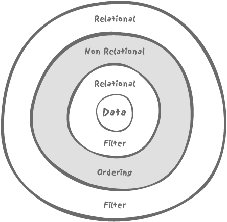
where rownum <= 5So, how is our query layered in this case? Many would be tempted to say that by applying a filtering condition to an ordered result, we end up with something looking more or less like Figure 4-3.
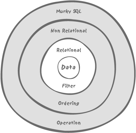
The truth, however, is more like Figure 4-4.
Using constructs that look relational doesn’t take us back to
the relational world, because to be in the relational world we must
apply relational operators to relations. Our subquery uses an order by to sort the results. Once we’ve
imposed ordering, we no longer have, strictly speaking, a relation (a
relation is a set, and a set has no order). We end up with an outer
select that looks relational on the
surface but is applied to the output of an inline view in which a
significant component (the order by
clause) is not a relational process.
My example of the top five nonexecutives is, of course, a simple example, but do understand that once we have left the relational sphere in the execution of a query, we can no longer return to it. The best we can possibly do is to use the output of such a query to feed into the relational phase of an outer query. For instance, “in which departments are our five top nonexecutive earners working?” What is extremely important to understand, though, is that at this stage no matter how clever the optimizer is, it will be absolutely unable to combine the queries, and will more or less have to execute them in a given sequence. Further, any resulting set from an intermediate query is likely to be held in temporary storage, whether in memory or on disk, where the choice of access methods may be reduced. Once outside the pure relational layer, the way we write a query is of paramount importance for performance because it will inevitably impose onto the query some execution path from which the SQL engine will not be able to stray.
To summarize, we can say that the safest approach we can adopt is to try to do as much of the job as possible inside the relational layer, where the optimizer can operate to maximum efficiency. When the situation is such that a given SQL task is no longer a purely relational problem, then we must be particularly careful about the construct, or the writing of the query itself. Understanding that SQL has, like Dr. Jekyll, a double nature is the key to mastering the language. If you see SQL as a single-edged sword, then you are condemned to remain in the world of tips and tricks for dummies, smarties, and mere mortals, possibly useful for impressing the opposite sex—although in my experience it doesn’t work much—but an approach that will never provide you with a deep understanding of how to cope with a difficult SQL problem.
Limits of the Optimizer
Any decent SQL engine relies heavily on its query optimizer, which very often performs an excellent job. However, there are many aspects of the way optimizers work that you must keep in mind:
- Optimizers rely on the information they find in the database.
This information is of two types: general statistical data (which must be verified as being fitting), and the essential declarative information held in the data definitions. Where important semantic information relating to the data relations is embedded in triggers or, worse, in application program code, that vital information will be totally unavailable to the optimizer. Such circumstances will inevitably impact the potential performance of the optimizer.
- Optimizers can perform to their best advantage where they can apply transformations that are mathematically proven to be equivalent.
When they are required to assess components of a query that are non-relational in character, they are on less certain grounds and the execution path will stick more closely to what was voluntarily or involuntarily suggested by the original writing.
- The work of the optimizer contributes to the overall response time.
Comparing a large number of alternative execution paths may take time. The end user sees only the total elapsed time and is unaware of how much was spent on optimization and how much on execution. A clever optimizer might allow itself more time to try to improve a query that it expects to take a lot of time to run, but there is always a self-imposed limit on its work. The trouble is that when you have a 20-way join (which is by no means unusual in some applications), the number of combinations the optimizer could examine can become unmanageably large even when adequate indexing make some links obvious. Compound this with the inclusion of a combination of complex views and subqueries, and at some point, the optimizer will have to give in. It is quite possible to find a situation in which a query running in isolation of any others may be very well optimized, while the same query deeply nested inside a much more complex outer query may take a completely wrong path.
- The optimizer improves individual queries.
It is unable to relate independent queries one to another, however. Whatever its efforts, if the bulk of your program is fetching data inside procedural code just to feed into subsequent queries, the optimizer will not be able to do anything for you.
Five Factors Governing the Art of SQL
You have seen in the first part of this chapter exactly how SQL includes both relational and non-relational characteristics. You have also seen how this affects the efficient (and not-so-efficient) workings of the database optimizer. From this point forward, and bearing in mind the lessons of the first part of this chapter, we can concentrate on the key factors that must be considered when using SQL. In my view, there are five main factors:
Total Quantity of Data
The volume of data we need to read is probably the most
important factor to take into account; an execution plan that is
perfectly suitable for a fourteen-row emp table and a four-row dept table may be entirely inappropriate for
dealing with a 15 million-row financial_flows table against which we have
to join a 5 million-row products
table. Note that even a 15 million-row table will not be considered
particularly large by the standards of many companies. As a matter of
consequence, it is hard to pronounce on the efficiency of a query
before having run it against the target volume of data.
Criteria Defining the Result Set
When we write an SQL statement, in most cases it will involve
filtering conditions located in where
clauses, and we may have several where clauses—a major one as well as minor
ones—in subqueries or views (regular views or in-line views). A
filtering condition may be efficient or inefficient. However, the
significance of efficient or
inefficient is strongly affected by other
factors, such as physical implementation (as discussed in Chapter 5) and once again, by how much
data we have to wade through.
We need to approach the subject of defining the result in several parts, by considering filtering, the central SQL statements, and the impact of large data volumes on our queries. But this is a particularly complex area that needs to be treated in some depth, so I’ll reserve this discussion until later in this chapter, in the major section entitled "Filtering.”
Size of the Result Set
An important and often overlooked factor is how much data a query returns (or how much data a statement changes). This is often dependent on the size of the tables and the details of the filtering, but not in every case. Typically, the combination of several selection criteria which of themselves are of little value in selecting data may result in highly efficient filtering when used in combination with one another. For example, one could cite that retrieving students’ names based on whether they received a science or an arts degree will give a large result set, but if both criteria are used (e.g., students who studied under both disciplines) the consequent result set will collapse to a tiny number.
In the case of queries in particular, the size of the result set
matters not so much from a technical standpoint, but mostly because of
the end user’s perception. To a very large extent, end users adjust
their patience to the number of rows they expect: when they ask for
one needle, they pay little attention to the size of the haystack. The
extreme case is a query that returns nothing, and a good developer
should always try to write queries that return few or no rows as fast
as possible. There are few experiences more frustrating than waiting
for several minutes before finally seeing a “no data found” message.
This is especially annoying if you have mistyped something, realized
your error just after hitting Enter, and then have been unable to
abort the query. End users are willing to wait to get a lot of data,
but not to get an empty result. If we consider that each of our
filtering criteria defines a particular result set and the final
result set is either the intersection (when conditions are anded) or the union (when conditions are
ored together) of all the
intermediate result sets , a zero result is most likely to result from the
intersection of small, intermediate result sets. In other words, the
(relatively) most precise criteria are usually the primary reason for
a zero result set. Whenever there is the slightest possibility that a
query might return no data, the most likely condition that would
result in a null return should be checked first—especially if it can
be done quickly. Needless to say, the order of evaluation of criteria
is extremely context-sensitive as you shall see later under "Filtering.”
Number of Tables
The number of tables involved in a query will naturally have some influence on performance. This is not because a DBMS engine performs joins badly—on the contrary, modern systems are able to join large numbers of tables very efficiently.
Joins
The perception of poor join performance is another enduring myth associated with relational databases. Folklore has it that one should not join too many tables, with five often suggested as the limit. In fact, you can quite easily have 15 table joins perform extremely well. But there are additional problems associated with joining a large number of tables, of which the following are examples:
When you routinely need to join, say, 15 tables, you can legitimately question the correctness of the design; keep in mind what I said in Chapter 1—that a row in a table states some kind of truth and can be compared to a mathematical axiom. By joining tables, we derive other truths. But there is a point at which we must decide whether something is an obvious truth that we can call an axiom, or whether it is a less obvious truth that we must derive. If we spend much of our time deriving our truths, perhaps our axioms are poorly chosen in the first place.
For the optimizer, the complexity increases exponentially as the number of tables increases. Once again, the excellent work usually performed by a statistical optimizer may comprise a significant part of the total response time for a query, particularly when the query is run for the first time. With large numbers of tables, it is quite impractical for the optimizer to explore all possible query paths. Unless a query is written in a way that eases the work of the optimizer, the more complex the query, the greater the chance that the optimizer will bet on the wrong horse.
When we write a complex query involving many tables, and when joins can be written in several fairly distinct ways, the odds are high that we’ll pick the wrong construct. If we join tables A to B to C to D, the optimizer may not have all the information present to know that A can be very efficiently joined directly to D, particularly if that join happens to be a special case. A sloppy developer trying to fix duplicate rows with a
distinctcan also easily overlook a missing join condition.
Complex queries and complex views
Be aware that the apparent number of tables involved in a query can be deceptive; some of the tables may actually be views, and sometimes pretty complex ones, too. Just as with queries, views can also have varying degrees of complexity. They can be used to mask columns, rows, or even a combination of rows and columns to all but a few privileged users. They can also be used as an alternate perspective on the data, building relations that are derived from the existing relations stored as tables. In cases such as these, a view can be considered shorthand for a query, and this is probably one of the most common usages of views. With increasingly complex queries, there is a temptation to break a query down into a succession of individual views, each representing a component of the greater query.
Like most extreme positions, it would be absurd to banish views altogether. Many of them are rather harmless animals. However, when a view is itself used in a rather complex query, in most cases we are only interested in a small fraction of the data returned by the view—possibly in a couple of columns, out of a score or more. The optimizer may attempt to recombine a simple view into a larger query statement. However, once a query reaches a relatively modest level of complexity, this approach may become too complex in itself to enable efficient processing.
In some cases a view may be written in a way that effectively
prevents the optimizer from combining it into the larger statement.
I have already mentioned rownums,
those virtual columns used in Oracle to indicate the order in which
rows are initially found. When rownums are used inside a view, a further
level of complexity is introduced. Any attempt to combine a view
that references a rownum into a
larger statement would be almost guaranteed to change the subsequent
rownum order, and therefore the
optimizer doesn’t permit a query rewrite in those circumstances. In
a complicated query, such a view will necessarily be executed in
isolation. In quite a number of cases then, the DBMS optimizer will
push a view as is into a statement,[*] running it as a step in the statement execution, and
using only those elements that are required from the result of the
view execution.
Frequently, many of the operations executed in a view
(typically joins to return a description associated with codes) will
be irrelevant in the context of a larger query, or a query may have
special search criteria that would have been particularly selective
when applied to the tables underlying the view. For instance, a
subsequent union may prove to be
totally unnecessary because the view is the union of several tables representing
subtypes, and the larger query filters on only one of the subtypes.
There is also the danger of joining a view with a table that itself
appears in the same view, thus forcing multiple passes over this
table and probably hitting the same rows several times when one pass
would have been quite sufficient.
When a view returns much more data than required in the context of a query that references that view, dramatic performance gains can often be obtained by eliminating the view (or using a simpler version of the view). Begin by replacing the view reference in the main query with the underlying SQL query used to define the view. With the components of the view in full sight, it becomes easy to remove everything that is not strictly necessary. More often than not, it’s precisely what isn’t necessary that prevents the view from being merged by the optimizer, and a simpler, cut-down view may give excellent results. When the query is correctly reduced to its most basic components, it runs much faster.
Many developers may hesitate to push the code for a very complex view into an already complex query, not least because it can make a complex situation even more complicated. The exercise of developing and factoring a complex SQL expression may indeed appear to be daunting. It is, however, an exercise quite similar to the development of mathematical expressions, as practiced in high school. It is, in my view, a very formative exercise and well worth the effort of mastering. It is a discipline that provides a very sound understanding of the inner workings of a query for developers anxious to improve their skills, and in most cases the results can be highly rewarding.
Number of Other Users
Finally, concurrency is a factor that you must carefully take into account when designing your SQL code. Concurrency is usually a concern while writing to the database where block-access contention , locking , latching (which means locking of internal DBMS resources), and others are the more obvious problem areas; even read consistency can in some cases lead to some degree of contention. Any server, no matter how impressive its specification, will always have a finite capacity. The ideal plan for a query running on a machine with little to no concurrency is not necessarily the same as the ideal plan for the same query running on the same machine with a high level of concurrency. Sorts may no longer find the memory they need and may instead resort to writing to disk, thus creating a new source of contention. Some CPU-intensive operations—for example, the computation of complicated functions, repetitive scanning of index blocks, and so forth—may cause the computer to overload. I have seen cases in which more physical I/Os resulted in a significantly better time to perform a given task. In those cases, there was a high level of concurrency for CPU-intensive operations, and when some processes had to wait for I/Os, the overworked CPUs were relieved and could run other processes, thus ensuring a better overlap. We must often think in terms of global throughput of one particular business task, rather than in terms of individual user response-time.
Note
Chapter 9 examines concurrency in greater detail.
Filtering
How you restrict your result set is one of the most critical
factors that helps you determine which tactics to apply when writing an
SQL statement. The collective criteria that filters the data are often
seen as a motley assortment of conditions associated in the where clause. However, you should very closely
examine the various where-clause (and
having-clause, too) conditions when
writing SQL code.
Meaning of Filtering Conditions
Given the syntax of the SQL language, it is quite
natural to consider that all filtering conditions , as expressed in the where clause, are similar in nature. This is
absolutely not the case. Some filtering conditions apply directly to
the select operator of relational
theory, where checking that a
column in a row (purists would say an attribute in a relation
variable) matches (or doesn’t match) a given condition. However,
historically the where clause also
contains conditions that implement another operator—the join operator. There is, since the advent of
the SQL92 join syntax, an attempt to differentiate join filtering conditions, located between
the (main) from clause and the
where clause, from the select filtering conditions listed in the
where clause. Joining two (or more)
tables logically creates a new relation.
Consider this general example of a join:
select .....
from t1
inner join t2
on t1.join1 = t2.joind2
where ...Should a condition on column c2 belonging to t2 come as an additional condition on the
inner join, expressing that in fact
you join on a subset of t2? Or
should a condition inside the where
clause, along with conditions on columns of t1, express that the filtering applies to
the result of joining t1 to
t2? Wherever you choose to place
your join condition ought not to
make much of a difference; however, it has been known to lead to
variations in performance with some optimizers.
We may also have conditions other than joins and the simple filtering of values. For instance, we may have conditions restricting the returned set of rows to some subtype; we may also have conditions that are just required to check the existence of something inside another table. All these conditions are not necessarily semantically identical, although the SQL syntax makes all of them look equivalent. In some cases, the order of evaluation of the conditions is of no consequence; in other cases, it is significant.
Here’s an example that you can actually find in more than one
commercial software package to illustrate the importance of the order
of the evaluation of conditions. Suppose that we have a parameters table, which holds: parameter_name, parameter_type, and parameter_value, with parameter_value being the string
representation of whatever type of parameter we have, as defined by
the attribute parameter_type. (To
the logical mind this is indeed a story of more woe than that of
Juliet and her Romeo, since the domain type of attribute parameter_value is a variable feast and thus
offends a primary rule of relational theory.) Say that we issue a
query such as:
select * from parameters
where parameter_name like '%size'
and parameter_type = 'NUMBER'With this query, it does not matter whether the first condition
is evaluated before or after the second one. However, if we add the
following condition, where int( )
is a function to convert from char
to integer value, then the order of
evaluation becomes very significant:
and int(parameter_value) > 1000
Now, the condition on parameter_type must be
evaluated before the condition on the value, because otherwise we risk
a run-time error consequent upon attempting to convert a character
string (if for example parameter_type for that row is defined as
char) to an integer. The optimizer may not be able to
figure out that the poor design demands that one condition should have
higher priority—and you may have trouble specifying it to the
database.
Evaluation of Filtering Conditions
The very first questions to consider when writing a SQL statement are:
What data is required, and from which tables?
What input values will we pass to the DBMS engine?
What are the filtering conditions that allow us to discard unwanted rows?
Be aware, however, that some data (principally data used for
joining tables) may be stored redundantly in several tables. A
requirement to return values known to be held in the primary key of a
given table doesn’t necessarily mean that this table must appear in
the from clause, since this primary
key may well appear as the foreign key of another table from which we
also need the data.
Even before writing a query, we should rank the filtering conditions. The really efficient ones (of which there may be several, and which may apply to different tables) will drive the query, and the inefficient ones will come as icing on the cake. What is the criterion that defines an efficient filter? Primarily, one that allows us to cut down the volume of the data we have to deal with as fast as possible. And here we must pay a lot of attention to the way we write; the following subsections work through a simple example to illustrate my point.
Buyers of Batmobiles
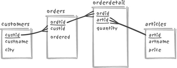
Assume that we have four tables, namely customers, orders, orderdetail, and a table of articles, as shown in Figure 4-5. Please note that
in the figure the sizes of the boxes representing each table are
more or less proportional to the volume of data in each table, not
simply to the number of columns. Primary key columns are
underlined.
Let’s now suppose that our SQL problem is to find the names of all the customers living in the city named “Gotham” who have ordered the article called “Batmobile” during the last six months. We have, of course, several ways to formulate this query; the following is probably what an ANSI SQL fan would write:
select distinct
c.custname
from customers c
join orders o
on o.custid = c.custid
join orderdetail od
on od.ordid = o.ordid
join articles a
on a.artid = od.artid
where c.city = 'GOTHAM'
and a.artname = 'BATMOBILE'
and o.ordered >= somefuncsomefunc is supposed to be a
function that returns the date six months prior to the current date.
Notice too, the presence of distinct, which may be required if one of
our customers is an especially heavy consumer of Batmobiles and has
recently ordered several of them.
Let’s forget for a while that the optimizer may rewrite the
query, and look at the execution plan such a statement suggests.
First, we walk the customers
table, keeping only rows for which the city happens to be Gotham.
Then we search the orders table,
which means that the custid
column there had better be indexed, because otherwise the only hope
the SQL engine has of executing the query reasonably fast is to
perform some sorting and merging or to scan the orders table to build a hash table and
then operate against that. We are going to apply another filter at
this level, against the order date. A clever optimizer will not mind
finding the filtering condition in the where clause and will understand that in
order to minimize the amount of data to join it must filter on the
date before performing the join. A not so clever optimizer might be
tempted to join first, and then filter, and may therefore be
grateful to you for specifying the filtering condition with the join
condition, as follows:
join orders o
on o.custid = c.custid
and o.ordered >= somefuncEven if the filtering condition really has nothing to do with
the join, it is sometimes difficult for the optimizer to understand
when that is the case. If the primary key of orderdetail is defined as (ordid, artid) then, because ordid is the first attribute of the index,
we can make use of that index to find the rows associated with an
order as in Chapter 3. But if
the primary key happens to be (artid,
ordid) (and note, either version is exactly the same as
far as relational theory is concerned), then tough luck. Some
products may be able to make some use of the index[*] in that case, but it will not provide the efficient
access that (ordid, artid) would
have allowed. Other products will be totally unable to use the
index. The only circumstance that may save us is the existence of a
separate index on ordid.
Once we have linked orderdetails to orders, we can proceed to articles—without any problem this time
since we found artid, the primary
key, in orderdetail. Finally, we
can check whether the value in articles is or is not a Batmobile. Is this
the end of the story? Not quite. As instructed by distinct, we must now sort the resulting
set of customer names that have passed across all the filtering
layers so as to eliminate duplicates.
It turns out that there are several alternative ways of expressing the query that I’ve just described. One example is to use the older join syntax , as follows:
select distinct c.custname
from customers c,
orders o,
orderdetail od,
articles a
where c.city = 'GOTHAM'
and c.custid = o.custid
and o.ordid = od.ordid
and od.artid = a.artid
and a.artname = 'BATMOBILE'
and o.ordered >= somefuncIt may just be old habits dying hard, but I prefer this older
way, if only for one simple reason: it makes it slightly more
obvious that from a logical point of view the order in which we
process data is arbitrary, because the same data will be returned
irrespective of the order in which we inspect tables. Certainly the
customers table is particularly
important, since that is the source from which we obtain the data
that is ultimately required, while in this very specific context,
all the other tables are used purely to support the remaining
selection processes. One really has to understand that there is no
one recipe that works for all cases. The pattern of table joins will
vary for each situation you encounter. The deciding factor is the
nature of the data you are dealing with.
A given approach in SQL may solve one problem, but make another situation worse. The way queries are written is a bit like a drug that may heal one patient but kill another.
More Batmobile purchases
Let’s explore alternative ways to list our buyers of
Batmobiles. In my view, as a general rule, distinct at the top level should be
avoided whenever possible. The reason is that if we have overlooked
a join condition, a distinct will
hide the problem. Admittedly this is a greater risk when building
queries with the older syntax, but nevertheless still a risk when
using the ANSI/SQL92 syntax if tables are joined through several
columns. It is usually much easier to spot duplicate rows than it is
to identify incorrect data.
It’s easy to give a proof of the assertion that incorrect
results may be difficult to spot: the two previous queries that use
distinct to return the names of
the customers may actually return a wrong result. If we happen to
have several customers named “Wayne,” we won’t get that information
because distinct will not only
remove duplicates resulting from multiple orders by the same
customer, but also remove duplicates resulting from homonyms. In
fact, we should return both the unique customer id and the customer
name to be certain that we have the full list of Batmobile buyers.
We can only guess at how long it might take to identify such an
issue in production.
How can we get rid of distinct then? By acknowledging that we
are looking for customers in Gotham that satisfy an existence
test , namely a purchase order for a Batmobile in the past
six months. Note that most, but not all, SQL dialects support the
following syntax:
select c.custname
from customers c
where c.city = 'GOTHAM'
and exists (select null
from orders o,
orderdetail od,
articles a
where a.artname = 'BATMOBILE'
and a.artid = od.artid
and od.ordid = o.ordid
and o.custid = c.custid
and o.ordered >= somefunc)If we use an existence test such as this query uses, a name
may appear more than once if it is common to several customers, but
each individual customer will appear only once, irrespective of the
number of orders they placed. You might think that my criticism of
the ANSI SQL syntax was a little harsh, since customers figure as prominently, if not
more prominently than before. However, it now features as the source
for the data we want the query to return. And another query, nested
this time, appears as a major phase in the identification of the
subset of customers.
The inner query in the preceding example is strongly linked to
the outer select. As you can see
on line 11 (in bold), the inner query refers to the current row of
the outer query. Thus, the inner query is what is called a
correlated subquery. The snag with this type of
subquery is that we cannot execute it before we know the current
customer. Once again, we are assuming that the optimizer doesn’t
rewrite the query. Therefore we must first find each customer and
then check for each one whether the existence test is satisfied. Our
query as a whole may perform excellently if we have very few
customers in Gotham. It may be dreadful if Gotham is the place where
most of our customers are located (a case in which a sophisticated
optimizer might well try to execute the query in a different
way).
We have still another way to write our query, which is as follows:
select custname
from customers
where city = 'GOTHAM'
and custid in
(select o.custid
from orders o,
orderdetail od,
articles a
where a.artname = 'BATMOBILE'
and a.artid = od.artid
and od.ordid = o.ordid
and o.ordered >= somefunc)In this case, the inner query no longer depends on the outer query: it has become an uncorrelated subquery. It needs to be executed only once. It should be obvious that we have now reverted the flow of execution. In the previous case, we had to search first for customers in the right location (e.g., where city is Gotham), and then check each order in turn. In this latest version of the query, the identifiers of customers who have ordered what we are looking for are obtained via a join that takes place in the inner query.
If you have a closer look, however, there are more subtle
differences as well between the current and preceding examples. In
the case of the correlated subquery, it is of paramount importance
to have the orders table indexed
on custid; in the second case, it
no longer matters, since then the index (if any) that will be used
is the index associated with the primary key of customers.
You might notice that the most recent version of the query
performs an implicit distinct. Indeed,
the subquery, because of its join, might return many rows for a
single customer. That duplication doesn’t matter, because the
in condition checks only to see
whether a value is in the list returned by the subquery, and
in doesn’t care whether a given
value is in that list one time or a hundred times. Perhaps though,
for the sake of consistency we should apply the same rules to the
subquery that we have applied to the query as a whole, namely to
acknowledge that we have an existence test within the subquery as
well:
select custname
from customers
where city = 'GOTHAM'
and custid in
(select o.custid
from orders o
where o.ordered >= somefunc
and exists (select null
from orderdetail od,
articles a
where a.artname = 'BATMOBILE'
and a.artid = od.artid
and od.ordid = o.ordid))or:
select custname
from customers
where city = 'GOTHAM'
and custid in
(select custid
from orders
where ordered >= somefunc
and ordid in (select od.ordid
from orderdetail od,
articles a
where a.artname = 'BATMOBILE'
and a.artid = od.artid)Irrespective of the fact that our nesting is getting deeper
and becoming less legible, choosing which query is the best between
the exists and the in follows the very same rule inside the
subquery as before: the choice depends on the effectiveness of the
condition on the date versus the condition on the article. Unless
business has been very, very slow for the past six months, one might
reasonably expect that the most efficient condition on which to
filter the data will be the one on the article name. Therefore, in
the particular case of the subquery, in is better than exists because it will be faster to find
all the order lines that refer to a Batmobile and then to check
whether the sale occurred in the last six months rather than the
other way round. This approach will be faster assuming that the
table orderdetail is indexed on
artid; otherwise, our bright,
tactical move will fail dismally.
Note
It may be a good idea to check in against exists whenever an existence test is
applied to a significant number of rows.
Most SQL dialects allow you to rewrite uncorrelated subqueries
as inline views in the from
clause. However, you must always remember that an in performs an implicit removal of
duplicate values, which must become explicit when the subquery is
moved to become an in-line view in the from clause. For example:
select custname
from customers
where city = 'GOTHAM'
and custid in
(select o.custid
from orders o,
(select distinct od.ordid
from orderdetail od,
articles a
where a.artname = 'BATMOBILE'
and a.artid = od.artid) x
where o.ordered >= somefunc
and x.ordid = o.ordid)The different ways you have to write functionally equivalent queries (and variants other than those given in this section are possible) are comparable to words that are synonyms. In written and spoken language, synonyms have roughly the same meaning, but each one introduces a subtle difference that makes one particular word more suitable to a particular situation or expression (and in some cases another synonym is totally inappropriate). In the same way, both data and implementation details may dictate the choice of one query variant over others.
Lessons to be learned from the Batmobile trade
The various examples of SQL that you saw in the
preceding section may look like an idle exercise in programming
dexterity, but they are more than that. The key point is that there
are many different ways in which we can attack the data, and that we
don’t necessarily have to go first through customers, then orders, then orderdetail, and then articles as some of the ways of writing
the query might suggest.
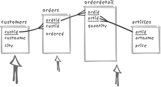
If we represent the strength of our search criteria with
arrows—the more discriminant the criterion, the larger the arrow—we
can assume that we have very few customers in Gotham, but that we
sell quite a number of Batmobiles and business has been brisk for
the past six months, in which case our battle map may look like
Figure 4-6. Although we
have a condition on the article name, the medium arrow points to
orderdetail because that is what
truly matters. We may have very few articles for sale, which may
represent similar percentages of our revenue, or we may have a huge
number of articles, of which one of the best sellers is the
Batmobile.
Alternatively, we can assume that most of our customers are
indeed based in Gotham, but that very few actually buy Batmobiles,
in which case our battle plan will look more like Figure 4-7. It is quite
obvious then, that we really have to cut to pieces the orderdetail table, which is the largest
one. The faster we slash this table, the faster our query will
run.

Note also—and this is a very important point—that the criterion “during the last six months” is not a very precise one. But what if we change the criterion to specify the last two months and happen to have 10 years of sales history online? In that case, it may be more efficient to get to those recent orders first—which, thanks to some techniques described in Chapter 5, may be clustered together—and then start from there, selecting customers from Gotham, on the one hand, and orders for Batmobiles on the other. To put it another way, the best execution plan does not only depend on the data values, it may also evolve over time.
What then can we conclude from all this? First, that there is more than one way to skin a cat...and that an expression of a query is usually associated with implicit assumptions about the data. With each different expression of a query we will obtain the same result set, but it may be at significantly different speeds. The way we write the query may influence the execution path, especially when we have to apply criteria that cannot be expressed within the truly relational part of the environment. If the optimizer is to be allowed to function at its best, we must try to maximize the amount of true relational processing and ensure the non-relational component has minimum impact on the final result.
We have assumed all along in this chapter that statements will be run as suggested by the way they are written. Be aware though, that an optimizer may rewrite queries—sometimes pretty aggressively. You could argue that rewrites by the optimizer don’t matter, because SQL is supposed to be a declarative language in which you state what you want and let the DBMS provide it. However, you have seen that each time we have rewritten a query in a different way, we have had to change assumptions about the distribution of data and about existing indexes. It is highly important, therefore, to anticipate the work of the optimizer to be certain that it will find what it needs, whether in terms of indexes or in terms of detailed-enough statistical information about the data.
Querying Large Quantities of Data
It may sound obvious, but the sooner we get rid of
unwanted data, the less we have to process at later stages of a
query—and the more efficiently the query will run. An excellent
application of this principle can be found with set operators, of
which union is probably the most
widely used. It is quite common to find in a moderately complex
union a number of tables appearing
in several of the queries “glued” together with the union operator. One often sees the union of fairly complex joins, with most of
the joined tables occurring in both select statements of the union—for example, on both sides of the
union, something like the
following:
select ...
from A,
B,
C,
D,
E1
where (condition on E1)
and (joins and other conditions)
union
select ...
from A,
B,
C,
D,
E2
where (condition on E2)
and (joins and other conditions)This type of query is typical of the cut-and-paste school of
programming. In many cases it may be more efficient to use a union of those tables that are not common,
complete with the screening conditions, and to then push that union into an inline view and join the
result, writing something similar to:
select ...
from A,
B,
C,
D,
(select ...
from E1
where (condition on E1)
union
select ...
from E2
where (condition on E2)) E
where (joins and other conditions)Another classic example of conditions applied at the wrong place
is a danger associated with filtering when a statement contains a
group by clause. You can filter on
the columns that define the grouping, or the result of the aggregate
(for instance when you want to check whether the result of a count( ) is smaller than a threshold) or
both. SQL allows you to specify all such conditions inside the
having clause that filters after
the group by (in practice, a sort
followed by an aggregation) has been completed. Any condition bearing
on the result of an aggregate function must be inside the having clause, since the result of such a
function is unknown before the group
by. Any condition that is independent on the aggregate
should go to the where clause and
contribute to decrease the number of rows that we shall have to sort
to perform the group by.
Let’s return to our customers and orders example, admitting that
the way we process orders is rather complicated. Before an order is
considered complete, we have to go through several phases that are
recorded in the table orderstatus,
of which the main columns are ordid, the identifier of the order; status; and statusdate, which is a timestamp. The
primary key is compound, consisting of ordid, and statusdate. Our requirement is to list, for
all orders for which the status is not flagged as complete (assumed to
be final), the identifier of the order, the customer name, the last
known order status, and when this status was set. To that end, we
might build the following query, filtering out completed orders and
identifying the current status as the latest status assigned:
select c.custname, o.ordid, os.status, os.statusdate
from customers c,
orders o,
orderstatus os
where o.ordid = os.ordid
and not exists (select null
from orderstatus os2
where os2.status = 'COMPLETE'
and os2.ordid = o.ordid)
and os.statusdate = (select max(statusdate)
from orderstatus os3
where os3.ordid = o.ordid)
and o.custid = c.custidAt first sight this query looks reasonable, but in fact it contains a number of deeply disturbing features. First, notice that we have two subqueries, and notice too that they are not nested as in the previous examples, but are only indirectly related to each other. Most worrying of all, both subqueries hit the very same table, already referenced at the outer level. What kind of filtering condition are we providing? Not a very precise one, as it only checks for the fact that orders are not yet complete.
How can such a query be executed? An obvious approach is to scan
the orders table, for each row
checking whether each order is or is not complete. (Note that we might
have been happy to find this information in the orders table itself,
but this is not the case.) Then, and only then, can we check the date
of the most recent status, executing the subqueries in the order in
which they are written.
The unpleasant fact is that both subqueries are correlated.
Since we have to scan the orders
table, it means that for every row from orders we shall have to check whether we
encounter the status set to COMPLETE for that order. The subquery to
check for that status will be fast to execute, but not so fast when
repeated a large number of times. When there is no COMPLETE status to be found, then a second
subquery must be executed. What about trying to un-correlate
queries?
The easiest query to un-correlate happens to be the second one. In fact, we can write, at least with some SQL dialects:
and (o.ordid, os.statusdate) = (select ordid, max(statusdate)
from orderstatus
group by ordid)The subquery that we have now will require a full scan of
orderstatus; but that’s not
necessarily bad, and we’ll discuss our reasoning in a moment.
There is something quite awkward in the condition of the pair of
columns on the left-hand side of the rewritten subquery condition.
These columns come from different tables, and they need not do so. In
fact, we want the order identifier to be the same in orders and orderstatus; will the optimizer understand
the subtlety of this situation? That is rather uncertain. If the
optimizer doesn’t understand, then it will be able to execute the
subquery first, but will have to join the two other tables together
before being able to exploit the result of the subquery. If the query
were written slightly differently, the optimizer would have greater
freedom to decide whether it actually wants to do what I’ve just
described or exploit the result of the subquery and then join orders to orderstatus:
    and (os.ordid, os.statusdate) = (select ordid, max(statusdate)
                                      from orderstatus
                                      group by ordid)
The reference on the left side to two columns from the same
table removes the dependence of identification of the most recent
status for the order on a preliminary join between orderstatus and orders. A very clever optimizer might have
performed the modification for us, but it is wiser to take no risk and
specify both columns from the same table to begin with. It is always
much better to leave the optimizer with as much freedom as we
can.
You have seen previously that an uncorrelated subquery can become a join in an inline view without much effort. We can indeed rewrite the entire query to list pending orders as follows:
    select c.custname, o.ordid, os.status, os.statusdate
    from customers c,
         orders o,
         orderstatus os,
         (select ordid, max(statusdate) laststatusdate
          from orderstatus
          group by ordid) x
    where o.ordid = os.ordid
      and not exists (select null
                      from orderstatus os2
                      where os2.status = 'COMPLETE'
                        and os2.ordid = o.ordid)
      and os.statusdate = x.laststatusdate
      and os.ordid = x.ordid
      and o.custid = c.custid
But then, if COMPLETE is
indeed the final status, do we need the subquery to check the
nonexistence of the last stage? The inline view helps us to identify
which is the last status, whether it is COMPLETE or anything else. We can apply a
perfectly satisfactory filter by checking the latest known
status:
    select c.custname, o.ordid, os.status, os.statusdate
    from customers c,
         orders o,
         orderstatus os,
         (select ordid, max(statusdate) laststatusdate
          from orderstatus
          group by ordid) x
    where o.ordid = os.ordid
      and os.statusdate = x.laststatusdate
      and os.ordid = x.ordid
      and os.status != 'COMPLETE'
      and o.custid = c.custid
The duplicate reference to orderstatus can be further avoided by using
OLAP or analytical functions available with some SQL engines. But
let’s pause here and consider how we have modified the query and, more
importantly, the execution path. Basically, our natural path was
initially to scan the orders table,
and then access through what may reasonably be expected to be an
efficient index on the table orderstatus. In the last version of our
query, we will attack through a full scan of orderstatus, to perform a group by. In terms of the number of rows,
orderstatus will necessarily be
several times bigger than orders.
However, in terms of mere volume of data to scan, we can expect it to
be smaller, possibly significantly smaller, depending on how much
information is stored for each order.
We cannot say with certainty which approach will be better, it
depends on the data. Let me add that seeing a full scan on a table
that is expected to grow is not a good idea (restricting the search to
the last month’s, or last few months’ worth of data can help). But
there are significant chances that this last version of our query will
perform better than the first attempt with the subquery in the
where clause.
We cannot leave the subject of large data volumes without mentioning a slightly special case. When a query returns a very large amount of data, you have reasonable grounds for suspecting that it’s not an individual sitting at a terminal that executed the query. The likelihood is that such a query is part of a batch process. Even if there is a longish “preparatory phase,” nobody will complain so long as the whole process performs to a satisfactory standard. Do not, of course, forget that a phase, preparatory or not, requires resources—CPU, memory, and possibly temporary disk space. It helps to understand that the optimizer, when returning a lot of data, may choose a path which has nothing in common with the path it would adopt when returning few rows, even if the fundamental query is identical.
The Proportions of Retrieved Data
A typical and frequently quoted saying is the famous “don’t use indexes when your query returns more than 10% of the rows of a table.” This states implicitly that (regular) indexes are efficient when an index key points to 10% or less of the rows in a table. As I have already pointed out in Chapter 3, this rule of thumb dates back to a time when relational databases were still regarded with suspicion in many companies. In those days, their use was mostly confined to that of departmental databases. This was a time when a 100,000-row table was considered a really big one. Compared to 10% of a 500 million-row table, 10% of 100,000 rows is a trifle. Can we seriously hope that the best execution plan in one case will still be the best execution plan in the other case? Such is wishful thinking.
Independently from the evolution of table sizes since the time when the “10% of rows” rule of thumb was first coined, be aware that the number of rows returned means nothing in itself, except in terms of response time expectations by end users. If you compute an average value over 1 billion rows, you return a single row, and yet the DBMS performs a lot of work. Even without any aggregation, what matters is the number of data pages that the DBMS is going to hit when performing the query. Data page hits don’t only depend on the existence of indexes: as you saw in Chapter 3, the relation of indexes to the physical order of rows in the table can make a significant difference in the number of pages to visit. Other implementation issues that I am going to discuss in Chapter 5 play an important part, too: depending on how data is physically stored, the same number of rows returned may mean that you have to visit massively different numbers of data pages. Furthermore, operations that would execute sequentially with one access path may be massively parallelized with another one. Don’t fall into the row percentage trap.
Get The Art of SQL now with the O’Reilly learning platform.
O’Reilly members experience books, live events, courses curated by job role, and more from O’Reilly and nearly 200 top publishers.

