Chapter 7. Case Study: Comparing Twitter Archives
One type of text that gets plenty of attention is text shared online via Twitter. In fact, several of the sentiment lexicons used in this book (and commonly used in general) were designed for use with and validated on tweets. Both authors of this book are on Twitter and are fairly regular users of it, so in this case study, let’s compare the entire Twitter archives of Julia and David.
Getting the Data and Distribution of Tweets
An individual can download his or her own Twitter archive by following directions available on Twitter’s website. We each downloaded ours and will now open them up. Let’s use the lubridate package to convert the string timestamps to date-time objects and initially take a look at our tweeting patterns overall (Figure 7-1).
library(lubridate)library(ggplot2)library(dplyr)library(readr)tweets_julia<-read_csv("data/tweets_julia.csv")tweets_dave<-read_csv("data/tweets_dave.csv")tweets<-bind_rows(tweets_julia%>%mutate(person="Julia"),tweets_dave%>%mutate(person="David"))%>%mutate(timestamp=ymd_hms(timestamp))ggplot(tweets,aes(x=timestamp,fill=person))+geom_histogram(position="identity",bins=20,show.legend=FALSE)+facet_wrap(~person,ncol=1)
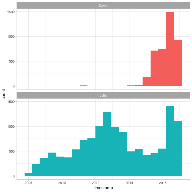
Figure 7-1. All tweets from our accounts
David and Julia tweet at about the same rate currently and joined Twitter about a year ...
Get Text Mining with R now with the O’Reilly learning platform.
O’Reilly members experience books, live events, courses curated by job role, and more from O’Reilly and nearly 200 top publishers.

