Chapter 1. The Tidy Text Format
Using tidy data principles is a powerful way to make handling data easier and more effective, and this is no less true when it comes to dealing with text. As described by Hadley Wickham (Wickham 2014), tidy data has a specific structure:
-
Each variable is a column.
-
Each observation is a row.
-
Each type of observational unit is a table.
We thus define the tidy text format as being a table with one token per row. A token is a meaningful unit of text, such as a word, that we are interested in using for analysis, and tokenization is the process of splitting text into tokens. This one-token-per-row structure is in contrast to the ways text is often stored in current analyses, perhaps as strings or in a document-term matrix. For tidy text mining, the token that is stored in each row is most often a single word, but can also be an n-gram, sentence, or paragraph. In the tidytext package, we provide functionality to tokenize by commonly used units of text like these and convert to a one-term-per-row format.
Tidy data sets allow manipulation with a standard set of “tidy” tools, including popular packages such as dplyr (Wickham and Francois 2016), tidyr (Wickham 2016), ggplot2 (Wickham 2009), and broom (Robinson 2017). By keeping the input and output in tidy tables, users can transition fluidly between these packages. We’ve found these tidy tools extend naturally to many text analyses and explorations.
At the same time, the tidytext package doesn’t expect a user to keep
text data in a tidy form at all times during an analysis. The package
includes functions to tidy() objects (see the broom package [Robinson, cited above]) from popular text mining R packages such as tm (Feinerer et al. 2008) and quanteda (Benoit and Nulty 2016). This
allows, for example, a workflow where importing, filtering, and
processing is done using dplyr and other tidy tools, after which the
data is converted into a document-term matrix for machine learning
applications. The models can then be reconverted into a tidy form for
interpretation and visualization with ggplot2.
Contrasting Tidy Text with Other Data Structures
As we stated above, we define the tidy text format as being a table with one token per row. Structuring text data in this way means that it conforms to tidy data principles and can be manipulated with a set of consistent tools. This is worth contrasting with the ways text is often stored in text mining approaches:
- String
-
Text can, of course, be stored as strings (i.e., character vectors) within R, and often text data is first read into memory in this form.
- Corpus
-
These types of objects typically contain raw strings annotated with additional metadata and details.
- Document-term matrix
-
This is a sparse matrix describing a collection (i.e., a corpus) of documents with one row for each document and one column for each term. The value in the matrix is typically word count or tf-idf (see Chapter 3).
Let’s hold off on exploring corpus and document-term matrix objects until Chapter 5, and get down to the basics of converting text to a tidy format.
The unnest_tokens Function
Emily Dickinson wrote some lovely text in her time.
text<-c("Because I could not stop for Death -","He kindly stopped for me -","The Carriage held but just Ourselves -","and Immortality")text
## [1] "Because I could not stop for Death -"   "He kindly stopped for me -"
## [3] "The Carriage held but just Ourselves -" "and Immortality"
This is a typical character vector that we might want to analyze. In order to turn it into a tidy text dataset, we first need to put it into a data frame.
library(dplyr)text_df<-data_frame(line=1:4,text=text)text_df
## # A tibble: 4 × 2
##    line                                   text
##   <int>                                  <chr>
## 1     1   Because I could not stop for Death -
## 2     2             He kindly stopped for me -
## 3     3 The Carriage held but just Ourselves -
## 4     4                        and Immortality
What does it mean that this data frame has printed out as a “tibble”? A tibble is a modern class of data frame within R, available in the dplyr and tibble packages, that has a convenient print method, will not convert strings to factors, and does not use row names. Tibbles are great for use with tidy tools.
Notice that this data frame containing text isn’t yet compatible with tidy text analysis. We can’t filter out words or count which occur most frequently, since each row is made up of multiple combined words. We need to convert this so that it has one token per document per row.
Note
A token is a meaningful unit of text, most often a word, that we are interested in using for further analysis, and tokenization is the process of splitting text into tokens.
In this first example, we only have one document (the poem), but we will explore examples with multiple documents soon.
Within our tidy text framework, we need to both break the text into
individual tokens (a process called tokenization) and transform it
to a tidy data structure. To do this, we use the tidytext
unnest_tokens() function.
library(tidytext)text_df%>%unnest_tokens(word,text)
## # A tibble: 20 × 2
##     line    word
##    <int>   <chr>
## 1      1 because
## 2      1       i
## 3      1   could
## 4      1     not
## 5      1    stop
## 6      1     for
## 7      1   death
## 8      2      he
## 9      2  kindly
## 10     2 stopped
## # ... with 10 more rows
The two basic arguments to unnest_tokens used here are column names.
First we have the output column name that will be created as the text is
unnested into it (word, in this case), and then the input column that
the text comes from (text, in this case). Remember that text_df
above has a column called text that contains the data of interest.
After using unnest_tokens, we’ve split each row so that there is one
token (word) in each row of the new data frame; the default tokenization
in unnest_tokens() is for single words, as shown here. Also notice:
-
Other columns, such as the line number each word came from, are retained.
-
Punctuation has been stripped.
-
By default,
unnest_tokens()converts the tokens to lowercase, which makes them easier to compare or combine with other datasets. (Use theto_lower = FALSEargument to turn off this behavior).
Having the text data in this format lets us manipulate, process, and visualize the text using the standard set of tidy tools, namely dplyr, tidyr, and ggplot2, as shown in Figure 1-1.

Figure 1-1. A flowchart of a typical text analysis using tidy data principles. This chapter shows how to summarize and visualize text using these tools.
Tidying the Works of Jane Austen
Let’s use the text of Jane Austen’s six completed, published novels from
the janeaustenr package
(Silge 2016), and transform them into a tidy format. The janeaustenr
package provides these texts in a one-row-per-line format, where a line
in this context is analogous to a literal printed line in a physical
book. Let’s start with that, and also use mutate() to annotate a
linenumber quantity to keep track of lines in the original format, and
a chapter (using a regex) to find where all the chapters are.
library(janeaustenr)library(dplyr)library(stringr)original_books<-austen_books()%>%group_by(book)%>%mutate(linenumber=row_number(),chapter=cumsum(str_detect(text,regex("^chapter [\\divxlc]",ignore_case=TRUE))))%>%ungroup()original_books
## # A tibble: 73,422 × 4
##                     text                book linenumber chapter
##                    <chr>              <fctr>      <int>   <int>
## 1  SENSE AND SENSIBILITY Sense & Sensibility          1       0
## 2                        Sense & Sensibility          2       0
## 3         by Jane Austen Sense & Sensibility          3       0
## 4                        Sense & Sensibility          4       0
## 5                 (1811) Sense & Sensibility          5       0
## 6                        Sense & Sensibility          6       0
## 7                        Sense & Sensibility          7       0
## 8                        Sense & Sensibility          8       0
## 9                        Sense & Sensibility          9       0
## 10             CHAPTER 1 Sense & Sensibility         10       1
## # ... with 73,412 more rows
To work with this as a tidy dataset, we need to restructure it in the
one-token-per-row format, which as we saw earlier is done with the
unnest_tokens() function.
library(tidytext)tidy_books<-original_books%>%unnest_tokens(word,text)tidy_books
## # A tibble: 725,054 × 4
##                   book linenumber chapter        word
##                 <fctr>      <int>   <int>       <chr>
## 1  Sense & Sensibility          1       0       sense
## 2  Sense & Sensibility          1       0         and
## 3  Sense & Sensibility          1       0 sensibility
## 4  Sense & Sensibility          3       0          by
## 5  Sense & Sensibility          3       0        jane
## 6  Sense & Sensibility          3       0      austen
## 7  Sense & Sensibility          5       0        1811
## 8  Sense & Sensibility         10       1     chapter
## 9  Sense & Sensibility         10       1           1
## 10 Sense & Sensibility         13       1         the
## # ... with 725,044 more rows
This function uses the tokenizers package to separate each line of text in the original data frame into tokens. The default tokenizing is for words, but other options include characters, n-grams, sentences, lines, paragraphs, or separation around a regex pattern.
Now that the data is in one-word-per-row format, we can manipulate it
with tidy tools like dplyr. Often in text analysis, we will want to
remove stop words, which are words that are not useful for an
analysis, typically extremely common words such as “the,” “of,”
“to,” and so forth in English. We can remove stop words (kept in the
tidytext dataset stop_words) with an anti_join().
data(stop_words)tidy_books<-tidy_books%>%anti_join(stop_words)
The stop_words dataset in the tidytext package contains stop words
from three lexicons. We can use them all together, as we have here, or
filter() to only use one set of stop words if that is more appropriate
for a certain analysis.
We can also use dplyr’s count() to find the most common words in all
the books as a whole.
tidy_books%>%count(word,sort=TRUE)
## # A tibble: 13,914 × 2
##      word     n
##     <chr> <int>
## 1    miss  1855
## 2    time  1337
## 3   fanny   862
## 4    dear   822
## 5    lady   817
## 6     sir   806
## 7     day   797
## 8    emma   787
## 9  sister   727
## 10  house   699
## # ... with 13,904 more rows
Because we’ve been using tidy tools, our word counts are stored in a tidy data frame. This allows us to pipe directly to the ggplot2 package, for example to create a visualization of the most common words (Figure 1-2).
library(ggplot2)tidy_books%>%count(word,sort=TRUE)%>%filter(n>600)%>%mutate(word=reorder(word,n))%>%ggplot(aes(word,n))+geom_col()+xlab(NULL)+coord_flip()
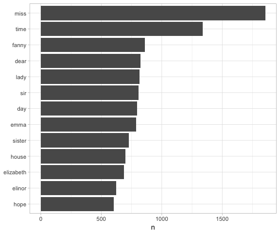
Figure 1-2. The most common words in Jane Austen’s novels
Note that the austen_books() function started us with exactly the text
we wanted to analyze, but in other cases we may need to perform cleaning
of text data, such as removing copyright headers or formatting. You’ll
see examples of this kind of pre-processing in the case study chapters,
particularly “Preprocessing”.
The gutenbergr Package
Now that we’ve used the janeaustenr package to explore tidying text,
let’s introduce the
gutenbergr package (Robinson
2016). The gutenbergr package provides access to the public domain works
from the Project Gutenberg collection. The
package includes tools both for downloading books (stripping out the
unhelpful header/footer information), and a complete dataset of Project
Gutenberg metadata that can be used to find works of interest. In this
book, we will mostly use the gutenberg_download() function that
downloads one or more works from Project Gutenberg by ID, but you can
also use other functions to explore metadata, pair Gutenberg ID with
title, author, language, and so on, or gather information about authors.
Tip
To learn more about gutenbergr, check out the package’s tutorial at rOpenSci, where it is one of rOpenSci’s packages for data access.
Word Frequencies
A common task in text mining is to look at word frequencies, just like
we have done above for Jane Austen’s novels, and to compare frequencies
across different texts. We can do this intuitively and smoothly using
tidy data principles. We already have Jane Austen’s works; let’s get two
more sets of texts to compare to. First, let’s look at some science
fiction and fantasy novels by H.G. Wells, who lived in the late 19th and
early 20th centuries. Let’s get The
Time Machine, The War of the
Worlds, The Invisible Man,
and The Island of Doctor Moreau.
We can access these works using gutenberg_download() and the Project
Gutenberg ID numbers for each novel.
library(gutenbergr)hgwells<-gutenberg_download(c(35,36,5230,159))
tidy_hgwells<-hgwells%>%unnest_tokens(word,text)%>%anti_join(stop_words)
Just for kicks, what are the most common words in these novels of H.G. Wells?
tidy_hgwells%>%count(word,sort=TRUE)
## # A tibble: 11,769 × 2
##      word     n
##     <chr> <int>
## 1    time   454
## 2  people   302
## 3    door   260
## 4   heard   249
## 5   black   232
## 6   stood   229
## 7   white   222
## 8    hand   218
## 9    kemp   213
## 10   eyes   210
## # ... with 11,759 more rows
Now let’s get some well-known works of the Brontë sisters, whose lives
overlapped with Jane Austen’s somewhat, but who wrote in a rather
different style. Let’s get Jane
Eyre, Wuthering Heights,
The Tenant of Wildfell Hall,
Villette, and
Agnes Grey. We will again use
the Project Gutenberg ID numbers for each novel and access the texts
using gutenberg_download().
bronte<-gutenberg_download(c(1260,768,969,9182,767))
tidy_bronte<-bronte%>%unnest_tokens(word,text)%>%anti_join(stop_words)
What are the most common words in these novels of the Brontë sisters?
tidy_bronte%>%count(word,sort=TRUE)
## # A tibble: 23,051 × 2
##      word     n
##     <chr> <int>
## 1    time  1065
## 2    miss   855
## 3     day   827
## 4    hand   768
## 5    eyes   713
## 6   night   647
## 7   heart   638
## 8  looked   602
## 9    door   592
## 10   half   586
## # ... with 23,041 more rows
Interesting that “time,” “eyes,” and “hand” are in the top 10 for both H.G. Wells and the Brontë sisters.
Now, let’s calculate the frequency for each word in the works of Jane
Austen, the Brontë sisters, and H.G. Wells by binding the data frames
together. We can use spread and gather from tidyr to reshape our
data frame so that it is just what we need for plotting and comparing the
three sets of novels.
library(tidyr)frequency<-bind_rows(mutate(tidy_bronte,author="Brontë Sisters"),mutate(tidy_hgwells,author="H.G. Wells"),mutate(tidy_books,author="Jane Austen"))%>%mutate(word=str_extract(word,"[a-z']+"))%>%count(author,word)%>%group_by(author)%>%mutate(proportion=n/sum(n))%>%select(-n)%>%spread(author,proportion)%>%gather(author,proportion,`Brontë Sisters`:`H.G. Wells`)
We use str_extract() here because the UTF-8 encoded texts from Project
Gutenberg have some examples of words with underscores around them to
indicate emphasis (like italics). The tokenizer treated these as words,
but we don’t want to count “any” separately from “any” as we saw
in our initial data exploration before choosing to use str_extract().
Now let’s plot (Figure 1-3).
library(scales)# expect a warning about rows with missing values being removedggplot(frequency,aes(x=proportion,y=`Jane Austen`,color=abs(`Jane Austen`-proportion)))+geom_abline(color="gray40",lty=2)+geom_jitter(alpha=0.1,size=2.5,width=0.3,height=0.3)+geom_text(aes(label=word),check_overlap=TRUE,vjust=1.5)+scale_x_log10(labels=percent_format())+scale_y_log10(labels=percent_format())+scale_color_gradient(limits=c(0,0.001),low="darkslategray4",high="gray75")+facet_wrap(~author,ncol=2)+theme(legend.position="none")+labs(y="Jane Austen",x=NULL)
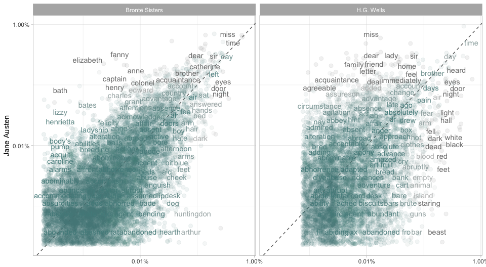
Figure 1-3. Comparing the word frequencies of Jane Austen, the Brontë sisters, and H.G. Wells
Words that are close to the line in these plots have similar frequencies in both sets of texts, for example, in both Austen and Brontë texts (“miss,” “time,” and “day” at the high frequency end) or in both Austen and Wells texts (“time,” “day,” and “brother” at the high frequency end). Words that are far from the line are words that are found more in one set of texts than another. For example, in the Austen-Brontë panel, words like “elizabeth,” “emma,” and “fanny” (all proper nouns) are found in Austen’s texts but not much in the Brontë texts, while words like “arthur” and “dog” are found in the Brontë texts but not the Austen texts. In comparing H.G. Wells with Jane Austen, Wells uses words like “beast,” “guns,” “feet,” and “black” that Austen does not, while Austen uses words like “family”, “friend,” “letter,” and “dear” that Wells does not.
Overall, notice in Figure 1-3 that the words in the Austen-Brontë panel are closer to the zero-slope line than in the Austen-Wells panel. Also notice that the words extend to lower frequencies in the Austen-Brontë panel; there is empty space in the Austen-Wells panel at low frequency. These characteristics indicate that Austen and the Brontë sisters use more similar words than Austen and H.G. Wells. Also, we see that not all the words are found in all three sets of texts, and there are fewer data points in the panel for Austen and H.G. Wells.
Let’s quantify how similar and different these sets of word frequencies are using a correlation test. How correlated are the word frequencies between Austen and the Brontë sisters, and between Austen and Wells?
cor.test(data=frequency[frequency$author=="Brontë Sisters",],~proportion+`Jane Austen`)
##
##  Pearson's product-moment correlation
##
## data:  proportion and Jane Austen
## t = 119.64, df = 10404, p-value < 2.2e-16
## alternative hypothesis: true correlation is not equal to 0
## 95 percent confidence interval:
##  0.7527837 0.7689611
## sample estimates:
##       cor
## 0.7609907
cor.test(data=frequency[frequency$author=="H.G. Wells",],~proportion+`Jane Austen`)
##
##  Pearson's product-moment correlation
##
## data:  proportion and Jane Austen
## t = 36.441, df = 6053, p-value < 2.2e-16
## alternative hypothesis: true correlation is not equal to 0
## 95 percent confidence interval:
##  0.4032820 0.4446006
## sample estimates:
##      cor
## 0.424162
Just as we saw in the plots, the word frequencies are more correlated between the Austen and Brontë novels than between Austen and H.G. Wells.
Summary
In this chapter, we explored what we mean by tidy data when it comes to text, and how tidy data principles can be applied to natural language processing. When text is organized in a format with one token per row, tasks like removing stop words or calculating word frequencies are natural applications of familiar operations within the tidy tool ecosystem. The one-token-per-row framework can be extended from single words to n-grams and other meaningful units of text, as well as to many other analysis priorities that we will consider in this book.
Get Text Mining with R now with the O’Reilly learning platform.
O’Reilly members experience books, live events, courses curated by job role, and more from O’Reilly and nearly 200 top publishers.

