Technical Mathematics, Sixth Edition

21.5. The Normal Curve

In the preceding section we showed some discrete probability distributions and studied the binomial distribution, one of the most useful of the discrete distributions. Now we introduce continuous probabilities and go on to study the most useful of these, the normal curve.

21.5.1. Continuous Probability Distributions

Suppose now that we collect data from a "large" population. For example, suppose that we record the weight of every college student in a certain state. Since the population is large, we can use very narrow class widths and still have many observations that fall within each class. If we do so, our relative frequency histogram, Fig. 21-12(a), will have very narrow bars, and our relative frequency polygon, Fig. 21-12(b), will be practically a smooth curve.

Figure 21.12. FIGURE 21-12

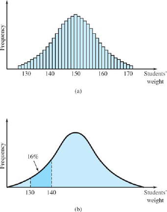
We get probabilities from the nearly smooth curve just as we did from the relative frequency histogram. The probability of an observation falling between two limits a and b is proportional to the area bounded by the curve and the x axis, between those limits. Let us designate the total area under the curve as 100% (or P = 1). Then the probability of an observation falling between two limits is equal to the area between those two limits.

Example 50: Suppose that 16% of the entire area under the curve in Fig. 21-12(b) lies between the limits 130 and 140. That means ...