Technical Mathematics, Sixth Edition

5.5. Solving an Equation Graphically

▪ Exploration: Try this.

1. Solve the equation x² − 1 = 0. What roots do you get?

2. Graph the equation y = x² − 1 for values of x from −3 to +3. What do you observe? Can you draw a tentative conclusion from your findings from steps (a) and (b)?

We can use our knowledge of graphing functions to solve equations of the form f(x) = 0. We mentioned earlier that a point at which a graph of a function y = f(x) crosses or touches the x axis is called an x intercept.

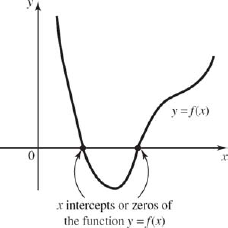
In Fig. 5-26 there are two zeros, since there are two x values for which y = 0, and hence f(x) = 0. Those x values for which f(x) = 0 are called zeros, roots or solutions to the equation f(x) = 0.

Thus if we were to graph the function y = f(x) any value of x at which y is equal to zero would be a solution to f(x) = 0. So to solve an equation graphically, we simply put it into the form f(x) = 0 and then graph the function y = f(x). Each x intercept is then an approximate solution to the equation.

Figure 5.26. FIGURE 5-26

Example 22: Graphically find the approximate root(s) of the equation 4.1x3 − 5.9x2 − 3.8x + 7.5 = 0 Solution: Let us represent the left side of the given equation by f(x). f(x) = 4.1x3 − 5.9x2 − 3.8x + 7.5 f(x). Any value of x for which f(x) = 0 will be a solution to Equation (1), so we f(x) simply graph and look for the x intercepts. The graph can be made manually as was shown ...