CHAPTER 20
CHAPTER 20 SOLUTIONS
20.1 SECTION 20.1
20.1 The first seven values of the cumulative distribution function for a Poisson(3) variable are 0.0498, 0.1991, 0.4232, 0.6472, 0.8153, 0.9161, and 0.9665. With 0.0498 ≤ 0.1247 < 0.1991, the first simulated value is x = 1. With 0.9161 ≤ 0.9321 < 0.9665, the second simulated value is x = 6. With 0.6472 ≤ 0.6873 < 0.8153, the third simulated value is x = 4.
20.2 The cumulative distribution function is
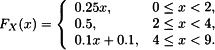
For u = 0.2, solve 0.2 = 0.25x for x = 0.8. The function is constant at 0.5 from 2 to 4, so the second simulated value is x = 4. For the third value, solve 0.7 = 0.1x + 0.1 for x = 6.
20.2 SECTION 20.2
20.3 Because 0.372 < 0.4, the first value is from the Pareto distribution. Solve ![]() for x = 100 [(1 − 0.693)−1/3 − 1] = 48.24. Because 0.702 ≥ 0.4, the second value is from the inverse Weibull distribution. Solve 0.284 = e−(200/x)2 for x = 200[− ln(0.284)]−1/2 = 178.26.
for x = 100 [(1 − 0.693)−1/3 − 1] = 48.24. Because 0.702 ≥ 0.4, the second value is from the inverse Weibull distribution. Solve 0.284 = e−(200/x)2 for x = 200[− ln(0.284)]−1/2 = 178.26.
20.4 For the first year, the number who remain employees is bin(200, 0.90) and the inversion method produces a simulated value of 175. The number alive but no longer employed is bin(25, 0.08/0.10 = 0.80) and the simulated value is 22. The remaning 3 employees die during the year. For year 2, the number who remain employed is bin(175, 0.90) and the simulated value ...
Get Student Solutions Manual to Accompany Loss Models: From Data to Decisions, Fourth Edition now with the O’Reilly learning platform.
O’Reilly members experience books, live events, courses curated by job role, and more from O’Reilly and nearly 200 top publishers.

