Statistical Inference for Models with Multivariate t-Distributed Errors

CHAPTER 4

SIMPLE REGRESSION MODEL

Outline

4.1 Introduction

4.2 Estimation and Testing of η

4.3 Properties of Intercept Parameter

4.4 Comparison

4.5 Numerical Illustration

4.6 Problems

In this chapter, we discuss some of the basic results from a simple regression model under the assumption that the error-vector is distributed according to the multivariate t-distribution. For normal errors see Saleh (2006) and for t-errors see Khan and Saleh (1997, 2008).

4.1 Introduction

Consider a simple linear model

(4.1.1)

where Y = (Y₁, Y₂, …, Y_n)′ is the response vector and x = (x₁, x₂, …, x_n)′ is a fixed vector of known constants, while ε = (ε₁, ε₂, …, ε_n)′ is the error vector distributed according to the low belonging to the class of multivariate t-distributions, say, M⁽ⁿ⁾_t (0, σ²V_n, γ_o).

As in Chapter 3, the covariance matrix is formulated as

(4.1.2)

4.2 Estimation and Testing of η

In this section, we consider LSE of η and test of hypothesis, H₀ : η = η_o vs H_A : η ≠ η_o.

4.2.1 Estimation of η

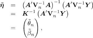
For the LSE of η, we minimize

to obtain the LSE of η as

(4.2.1)

where

(4.2.2)

with K₁ = 1′V⁻¹_n1, K