2.3 Tabular and Graphical Techniques: Grouped Data
The preceding set of descriptive techniques (tabular and graphical) was easily applied to discrete sets of data with a relatively small number of observations. (A small sample in statistics typically has about 30 observations (give or take a few data points) whereas a medium-sized sample has around 50 observations.) Much larger data sets, involving either discrete or continuous observations, can be handled in a much more efficient manner. That is, instead of listing each and every different value of some variable X (there may be hundreds of them) and then finding its associated absolute or relative frequency or percent, we can opt to group the values of X into specified classes.
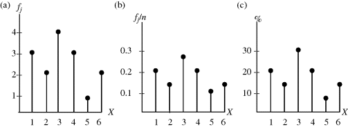
Figure 2.1 (a) Absolute frequency function. (b) Relative frequency function. (c) Percent function.

Paralleling the above development of tabular and graphical methods, let us first determine an absolute frequency distribution—it shows the absolute frequencies with which the various values of a variable X are distributed among chosen classes. Here an absolute frequency is now a class frequency—it is the number of items falling into a given class.
The process of constructing this distribution consists of the following steps:
Get Statistical Inference: A Short Course now with the O’Reilly learning platform.
O’Reilly members experience books, live events, courses curated by job role, and more from O’Reilly and nearly 200 top publishers.

