It’s been a hard day’s night And I’ve been working like a dog
—John Lennon and Paul McCartney: “A Hard Day’s Night” (1964)
Having defined the relvars in the suppliers-and-parts database (see Chapter 3), and having “loaded” or initialized them (again, see Chapter 3), we can now start to use them for “real work.” More specifically, we can now issue queries—i.e., retrieval requests—against those relvars, using operators of what’s called the relational algebra, and in this chapter I want to start our investigation into those operators. Caveat: The chapter is, regrettably, quite long, and you might want to take it a piece at a time. To help you in this regard, I haven’t left all of the exercises and answers to the very end of the chapter but have instead interspersed them at intervals among the regular explanatory text.
The relational algebra consists of a set of operators that (speaking very loosely) allow us to derive “new” relations from “old” ones. Each such operator takes one or more relations as input and produces another relation as output. For example, the difference operator (MINUS, in Tutorial D) takes two relations as input and “subtracts” one from the other, to derive another relation as output. And it’s very important that the output is another relation (that’s the so called closure property of the relational algebra). The reason it’s so important is this: It allows us to write nested relational expressions. To spell the point out, since the output from every operation is the same kind of thing as the input, the output from one operation can become the input (or one of the inputs) to another. For example, we can take the difference r1 MINUS r2, feed the result as input to a union with some relation r3, feed that result as input to an intersection with some relation r4, and so on.
There’s an analogy here that might help, to do with ordinary arithmetic. In arithmetic, we can (for example) take the sum of two numbers a and b to obtain a result, c; and that output c is the same kind of thing as the input—they’re all numbers—and so we can take that output and feed it as input to, say, a multiplication operation; and then we can feed the result of that multiplication as input to a subtraction (and so on). In other words, numbers form a closed system under the regular arithmetic operators, and it’s that fact that allows us to write nested arithmetic expressions. Likewise, relations are closed under the operators of the relational algebra, and the significance is precisely analogous: As I’ve said, we can write nested relational expressions.
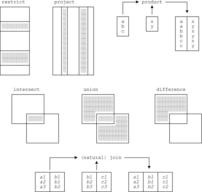
Now, any number of operators can be defined that fit the simple definition of “one or more relations in, exactly one relation out.” Below I briefly describe what are usually thought of as the original operators (essentially the ones that Codd defined in his earliest papers);[26] I’ll give more details of those operators in subsequent sections of the chapter, and then in Chapter 5 I’ll describe a number of additional operators. Figure 4-1 gives a pictorial representation of those original operators. Note: If you’re unfamiliar with these operators and find the descriptions in this preliminary section a little hard to understand, don’t worry about it. As I’ve already said, I’ll be going into much more detail, with lots of examples, later in the chapter.
- Restrict
Returns a relation containing all tuples from a specified relation that satisfy a specified condition. For example, we might restrict the suppliers relation to just those tuples where the STATUS value is less than 25.
- Project
Returns a relation containing all (sub)tuples that remain in a specified relation after specified attributes have been removed. (As noted in the answer to Q: in Chapter 3, a subtuple is still a tuple, just as—and indeed precisely because—a subset is still a set.) For example, we might project the suppliers relation on just the SNO and CITY attributes (thereby removing the SNAME and STATUS attributes).
- Product
Returns a relation containing all possible tuples that are a combination of two tuples, one from each of two specified relations. For example, let r1 be the projection of the suppliers relation on SNO and let r2 be the projection of the parts relation on PNO. Then—thanks to the closure property—we could form the product of r1 and r2, and the result would consist of all possible SNO-PNO pairs such that the SNO value is a supplier number appearing in the suppliers relation and the PNO value is a part number appearing in the parts relation. Note: “Product” here really means cartesian product, and the operator is sometimes so called.
- Intersect
Returns a relation containing all tuples that appear in both of two specified relations.
- Union
Returns a relation containing all tuples that appear in either or both of two specified relations.
- Difference
Returns a relation containing all tuples that appear in the first and not the second of two specified relations.
- Join
Returns a relation containing all possible tuples that are a combination of two tuples, one from each of two specified relations, such that the two tuples contributing to any given result tuple have common values for the common attributes of the two relations (and those common values appear just once, not twice, in that result tuple). Note: This kind of join was originally called the natural join, to distinguish it from various other kinds—especially the so called θ-join (“theta join”), to be discussed briefly in Chapter 11 in Part III of this book. Since natural join is far and away the most important kind, however, it’s become standard practice to take the unqualified term join to mean the natural join specifically, and I’ll follow that practice throughout this book.
Finally, there are a number of additional points I need to make before I close this section:
The operators of the algebra are generic: They apply, in effect, to all possible relations. For example, we don’t need one join operator to join (say) suppliers and shipments and another totally different join operator to join (say) departments and employees.
The operators are also set level, or (perhaps better) relation level: They take whole relations as operands, not individual tuples, and they return whole relations as their result.[27]
The operators are also read-only: They “read” their operands and they return a result, but they don’t update anything. In other words, they operate on relations, not relvars.
Of course, the previous point doesn’t mean that relational expressions can’t refer to relvars. For example, if R1 and R2 are relvar names, then R1 MINUS R2 is certainly a valid relational expression in Tutorial D (just so long as the relvars denoted by those names are of the same type, that is—see later). In that expression, however, R1 and R2 don’t denote those relvars as such; rather, they denote the relations that happen to be the current values of those relvars at the time the expression is evaluated. In other words, we can certainly use a relvar name to denote an operand to a relational algebra operator—and such a relvar reference thus constitutes one simple kind of relational expression—but in principle we could equally well denote the very same operand by means of an appropriate relation literal instead.
An analogy might help clarify this point. Suppose N is a variable of type INTEGER, and at time t it has the value 3. Then N + 2 is certainly a valid arithmetic expression, but at time t it means exactly the same as the expression 3 + 2 does, no more and no less.
Finally, given that the operators of the algebra are indeed all read-only, it follows that INSERT, DELETE, and UPDATE (and relational assignment), though they’re certainly relational operators, aren’t relational algebra operators as such—though, regrettably, you’ll often come across statements to the contrary in the literature. (In fact, of course, INSERT, DELETE, UPDATE, and relational assignment are all, specifically, update operators, whereas the algebraic operators are, as I’ve said, all read-only.)
Now we can begin to examine the operators of the algebra in more detail. I’ll start with restrict. Consider this query: “Get part information for parts whose weight is less than 12.5 pounds.” (I’m assuming here, just to be definite, that part weights are recorded in relvar P in pounds avoirdupois.) Here then is a Tutorial D formulation of this query:
P WHERE WEIGHT < 12.5
And here’s the result, given our usual sample values:[28]
|
|
|
|
|
|
|
|
|
|
|
|
|
|
|
As you can see, the result is certainly a relation; what’s more, the heading of that result is the same as that of the input (i.e., the parts relation, which is to say the current value of relvar P), and the body of that result consists of just those tuples of the input for which the specified restriction condition—viz., WEIGHT < 12.5—evaluates to TRUE.
Here then for the record is a precise definition of the restriction operator:
Definition: Let r be a relation and let bx be a restriction condition on r (i.e., a boolean expression in which every attribute reference identifies some attribute of r and there aren’t any relvar references). Then the expression r WHERE bx denotes the restriction of r according to bx, and it returns a relation with heading the same as that of r and body consisting of all tuples of r for which bx evaluates to TRUE.
Points arising from this definition:
The definition mentions the term restriction condition, defining it to be a boolean expression in which every attribute reference identifies some attribute of the pertinent relation and there aren’t any relvar references. (Note that the boolean expression in the example is indeed a restriction condition by this definition.) As you might have realized, the point about a boolean expression that takes this very simple form is that it can be evaluated for a given tuple of the pertinent relation “in isolation,” as it were—there’s no need to examine any other tuples in that relation, and there’s no need to examine any other relations, either. For example, the restriction condition WEIGHT < 12.5 can be determined to be true or false (as applicable) for a given tuple in the parts relation “in isolation” in exactly the foregoing sense.
To repeat, the boolean expression in the WHERE clause is supposed to be a restriction condition. As a matter of user convenience, however, real languages, including both Tutorial D and SQL in particular, usually allow WHERE clauses to contain boolean expressions that are more general than this. Examples are given in later chapters. Note: It’s legitimate to relax the strict requirement in this way because, if exp is an expression of the form r WHERE bx in which bx is not a restriction condition as such, then exp can always be shown to be equivalent to some more complicated expression in which any restrictions involved do in fact abide by the requirement after all.
It follows from the definition that the type of the result from a restriction operation is always the same as that of the input (since they both have the same heading).
Restriction is sometimes known as selection, but this latter term is deprecated, slightly, because of the potential confusion with (a) the SELECT operation of SQL (see Part III of this book) and (b) selector operators in the relational model (see Chapter 7).
Now on to project. Consider the query “For each part, get part number, color, and city.” Here’s a Tutorial D formulation:
P { PNO , COLOR , CITY }
|
|
|
|
|
|
|
|
|
|
|
|
|
|
|
|
|
|
|
|
|
As you can see, the result is a relation once again; its heading consists of the attributes specified in the projection, and its body consists of the corresponding (sub)tuples of the input.
Here’s another example, to illustrate another point. The query is “What part color and city combinations currently exist?” Tutorial D formulation:
P { COLOR , CITY }Here’s the result:
|
|
|
|
|
|
|
|
|
|
The point about this example is that the cardinality of the result is four, not six; even though there are six tuples in the input (the parts relation), three of those six contain the same color and city combination. Now, we want the result to be a relation—i.e., we want to preserve the closure property—and relations by definition never contain duplicate tuples; thus, those three tuples with the same color and city combination together contribute just one tuple to the overall result. In other words, “duplicates are eliminated,” to use the common phrase.
Aside: Observe that the result in this example is “all key,” meaning the sole key is the entire heading (note the double underlining in the picture). However, see Q: in the next chapter for further discussion of this point. End of aside.
By the way, I’d like to point out that it’s intuitively reasonable, as well as being logically correct, to do duplicate elimination in the foregoing example. Consider the original query once again: “What part color and city combinations currently exist?” Well, the combination “red and London” certainly exists; in fact, of course, it appears three times. But the query didn’t ask how many times that combination appeared, it merely asked whether it existed. And the right answer to a question of the form “Does x exist?” is either yes or no, not a count.[29]
Note: In principle duplicate elimination was done in the previous projection example too, but in that case it had no effect. And the reason it had no effect was that, in that example, the set of attributes on which the projection was being done included a key (actually the only key) of the underlying relvar. To jump ahead of myself for a moment, let me add that conceptually, at least, duplicate elimination is always done as part of the process of producing the result of some algebraic operator. In practice, however, the only operators (out of the ones discussed in this chapter) for which duplicate elimination might actually be required—i.e., might actually have some effect on the result—are projection, which is the topic of the present section, and union, to be discussed later in the chapter.
Here then is a definition of the projection operator:
Definition: Let relation r have attributes called A1, A2, ..., An (and possibly others). Then the expression r{A1, A2, ..., An} denotes the projection of r on {A1, A2, ..., An}, and it returns a relation with heading {A1, A2, ..., An} and body consisting of all tuples t such that there exists a tuple in r that has the same value for attributes A1, A2, ..., An as t does.
Points arising from this definition:
Of course, the order in which the attributes are specified in a projection operation is irrelevant. That’s why the commalist of attribute names is enclosed in braces.[30] Thus, for example, these two expressions are logically equivalent and therefore effectively interchangeable:
P { COLOR , CITY }P { CITY , COLOR }As a matter of user convenience, Tutorial D also allows projection operations to be expressed in terms of the attributes to be removed instead of the ones to be retained. For example, the two projection examples discussed so far in this section could alternatively have been formulated in Tutorial D as follows:
P { ALL BUT PNAME , WEIGHT }P { ALL BUT PNO , PNAME , WEIGHT }Note: Tutorial D allows this ALL BUT style throughout the language (wherever it makes sense, in fact). In the VAR statement that defined relvar SP, for example, we could have specified KEY {ALL BUT QTY} instead of KEY {SNO,PNO}.
The type of the result from a projection operation is RELATION H, where the heading H consists of the attributes on which the projection was done. Note: In fact, of course, the type of the result of any relational operation is always RELATION H, where H is the applicable heading. Thus, I won’t bother to point this fact out explicitly any more.
Consider the query “Get part number, color, and city for parts whose weight is less than 12.5 pounds.” The obvious Tutorial D formulation is:
( P WHERE WEIGHT < 12.5 ) { PNO , COLOR , CITY }Here’s the result:
|
|
|
|
|
|
|
|
|
Note the use of parentheses, which forces the subexpression P WHERE WEIGHT < 12.5—which represents a restriction, of course—to be evaluated first. The result of that restriction is then projected on attributes PNO, COLOR, and CITY. So here we’re explicitly making use of closure again: The result of the restriction is a relation, and so it’s legitimate to perform a projection on it.
It follows from this example that when we say (as I did in the definition) that projection is denoted by an expression of the form r{A1, A2,..., An}, it’s important to understand that the symbol r in that expression itself represents a relational expression of, in general, arbitrary complexity. And, of course, the same goes for the symbol r in the restriction expression r WHERE bx, and more generally for any mention of a relation as such in any of the relational operator definitions.
4.1 The formal reason is simply that the body of a relation is defined to be a set, and sets in mathematics don’t permit duplicate elements. As for pragmatic reasons: Actually there are many, but we haven’t covered enough groundwork to explain most of them here. But there’s at least one that should make good intuitive sense, as follows.[31] Suppose “relvar” R permits duplicates. Then we can’t tell the difference between “genuine” (i.e., explicitly intended) duplicates in R and “accidental” ones (i.e., ones caused by some kind of user error). Nor can we easily delete those “accidental” ones, even if we can recognize them.
There’s another point too that applies specifically to the results of relational operations: If we don’t eliminate duplicates from those results, then those results won’t be relations, and we won’t be able to perform further relational operations to them. In other words, we’ll have violated closure, and we won’t be able to write proper nested expressions.
4.2 Now this is a complicated question, and I don’t think it has a simple, succinct answer.[32] Speaking a little loosely, however, an algebra can be defined as a formal system that consists of (a) a set of objects of some kind, together with (b) a set of read-only operators that apply to those objects, such that (c) those objects and operators together satisfy certain laws and properties, such as the closure property (see Appendix C). The word algebra itself derives from Arabic al-jebr, meaning a resetting (of something broken) or a combination. And relational algebra in particular does conform, somewhat, to the foregoing loose definition.
4.3 a. The projection of the relation that’s the current value of relvar SP on all of its attributes. The result is of course necessarily identical to that current value; indeed, a projection of a relation on all of its attributes is sometimes referred to as an identity projection for that very reason.
b. This expression—it’s a restriction expression, of course—returns the relation that’s the current value of relvar P, because the boolean expression in the WHERE clause evaluates to TRUE for every tuple in that current value. In fact, the restriction expression overall is logically equivalent to the restriction expression P WHERE TRUE. Note: Any restriction expression that’s logically equivalent to one of the form r WHERE TRUE is said to denote an identity restriction.
c. This expression (a restriction expression again) returns the empty parts relation. Any restriction expression that’s logically equivalent to one of the form r WHERE FALSE is said to denote an empty restriction.
Now I turn to union, intersection, and difference. These three operators all follow the same general pattern. I’ll start with union.
Consider the query “Get cities in which at least one supplier or at least one part is located.” Here’s a Tutorial D formulation (note the appeal to closure yet again):
S { CITY } UNION P { CITY }And here’s the result:
|
|
|
|
|
As you can see, the result is a relation once again; its heading is the same as that of each of the two input relations, and its body consists of tuples that appear in one or both of those two relations (with duplicates eliminated, as mentioned earlier). Note, therefore, that the two input relations must have the same heading—equivalently, they must be of the same type—for otherwise the union operation is undefined. But if it is defined, then the result too is of the same type as both of the inputs.
Here’s another example, to illustrate another (very simple) point. Suppose for the sake of the example that parts have an extra attribute called STATUS, of type INTEGER, and consider the query “Get status and city pairs such that at least one supplier or part has that combination.” In Tutorial D:
S { STATUS , CITY } UNION P { CITY , STATUS }The point of this example, of course, is simply that (as always) the left to right order in which attributes are specified within a heading is irrelevant.
Here then is a definition of the union operator:
Definition: Let relations r1 and r2 be of the same type T. Then the expression r1 UNION r2 denotes the union of r1 and r2, and it returns the relation of type T with body the set of all tuples t such that t appears in either or both of r1 and r2.
Intersection is very similar to union, mutatis mutandis; in particular, the two input relations must again be of the same type, and the result is of the same type also. Here’s an example (the query is “Get cities in which at least one supplier and at least one part are both located”). Tutorial D formulation:
S { CITY } INTERSECT P { CITY }Result:
|
|
|
Here’s the definition:
Definition: Let relations r1 and r2 be of the same type T. Then the expression r1 INTERSECT r2 denotes the intersection of r1 and r2, and it returns the relation of type T with body the set of all tuples t such that t appears in both r1 and r2.
Difference—MINUS in Tutorial D—is also somewhat similar to union; in particular, the two input relations must again be of the same type, and the result is of the same type also. Here’s an example (the query is “Get cities in which at least one supplier is located and no part is”). In Tutorial D:
S { CITY } MINUS P { CITY }Result:
|
|
There is, however, one point on which difference is not similar to union and intersection: Operand order matters. With union, r1 UNION r2 and r2 UNION r1 both mean the same thing; likewise, with intersection, r1 INTERSECT r2 and r2 INTERSECT r1 both mean the same thing. But with difference, r1 MINUS r2 and r2 MINUS r1 most definitely don’t mean the same thing, even if they return the same result (which can happen only if r1 and r2 are equal, in which case both results are empty). Thus, for example, the expression
P { CITY } MINUS S { CITY }evaluates to:
|
|
Here’s the definition:
Definition: Let relations r1 and r2 be of the same type T. Then the expression r1 MINUS r2 denotes the difference between r1 and r2 (in that order), and it returns the relation of type T with body the set of all tuples t such that t appears in r1 and not in r2.
The union operator in particular possesses a number of attractive formal properties that can help the user’s task of query formulation.[33] To be specific, the operator is commutative, associative, and idempotent. Commutative means r1 UNION r2 and r2 UNION r1 are equivalent (this property follows immediately from the fact that the definition of the operator is symmetric in r1 and r2); as already noted, therefore, the order in which the operands are specified makes no difference. Associative means r1 UNION (r2 UNION r3) and (r1 UNION r2) UNION r3 are equivalent, so the parentheses aren’t needed and both of these expressions can be simplified to just r1 UNION r2 UNION r3. Idempotent means r UNION r reduces to simply r.
The foregoing paragraph applies 100 percent, mutatis mutandis, to intersection also; that is, intersection too is commutative, associative, and idempotent. However, it doesn’t apply at all to difference, for which none of those three properties holds.
Consider the following query: “Get names such that at least one supplier or at least one part has the name in question.” (This query is very contrived and probably doesn’t make much intuitive sense, but it suffices to illustrate the point I want to make here.) Now, the following formulation doesn’t work:
S { SNAME } UNION P { PNAME }The reason it doesn’t work is that UNION requires its operands to be of the same type, meaning that corresponding attributes have to be of the same type and have the same name. (Formally, in fact, they have to be the very same attribute.) In order to meet this requirement in the case at hand, therefore, we must rename at least one of SNAME and PNAME before we do the union (these attributes are at least of the same type, but they obviously have different names). Here then is a possible formulation of the query that does work, in which, purely for reasons of symmetry, I’ve renamed both of the pertinent attributes:
( ( S RENAME { SNAME AS NAME } ) { NAME } )
  UNION
( ( P RENAME { PNAME AS NAME } ) { NAME } )
Before explaining in detail how this formulation works (if you haven’t figured it out for yourself already), let me discuss the RENAME operator as such.[34] Here’s the definition:
Definition: Let relation r have an attribute called A and no attribute called B. Then the expression r RENAME {A AS B} returns a relation with heading identical to that of r except that attribute A in that heading is renamed B, and body identical to that of r except that all references to A in that body—more precisely, in tuples in that body—are replaced by references to B.
And here’s an example:
S RENAME { CITY AS SCITY }The result looks like this (it’s identical to our usual suppliers relation, except that the city attribute is called SCITY):
|
|
|
|
|
|
|
|
|
|
|
|
|
|
|
|
|
|
|
|
|
|
|
|
Important: Relvar S has not been changed in the database here! The expression S RENAME {CITY AS SCITY} is only an expression (just as, e.g., r1 MINUS r2 or N + 2 are only expressions), and like any expression it simply denotes a value. What’s more, of course, since it is an expression and not a statement, it can be nested inside other expressions.
RENAME is needed primarily as a preliminary to a JOIN or UNION invocation.[35] The details of JOIN are still to be discussed, of course, but here again is the UNION example that introduced this section:
( ( S RENAME { SNAME AS NAME } ) { NAME } )
 UNION
( ( P RENAME { PNAME AS NAME } ) { NAME } )
Explanation:
The subexpression S RENAME {SNAME AS NAME} returns a relation essentially identical to the current value of relvar S, except that the SNAME attribute is renamed NAME. Let’s call that result r1. Relation r1 is then projected on NAME, to give as a result relation r2, say.
The subexpression P RENAME {PNAME AS NAME} returns a relation essentially identical to the current value of relvar P, except that the PNAME attribute is renamed NAME. Let’s call that result r3. Relation r3 is then projected on NAME, to give as a result relation r4, say.
Finally, the expression r2 UNION r4 is evaluated, to produce a relation of degree one, with sole attribute NAME (of type CHAR) and body consisting of all tuples of the form
TUPLE { NAME name }such that name appears as a value of the SNAME attribute in the current value of relvar S or a value of the PNAME attribute in the current value of relvar P or both.
4.4 Well, there are certainly no duplicates in the inputs, because the inputs are relations. Next, observe that r1 INTERSECT r2 can be loosely defined to mean “return the maximal subset r of r1 such that every tuple appearing in r also appears in r2”—from which it’s obvious that there aren’t any duplicates to be eliminated. Likewise, r1 MINUS r2 can be loosely defined to mean “return the maximal subset r of r1 such that no tuple appearing in r also appears in r2,” from which, again, it’s obvious that there aren’t any duplicates to be eliminated.
4.5 Let A and B be sets. Then the set theory union of A and B is the set of all elements appearing in at least one of A and B; the set theory intersection of A and B is the set of all elements appearing in both A and B; and the set theory difference between A and B, in that order, is the set of all elements appearing in A and not in B. See Appendix C for further discussion.
4.6 Note: My characterizations below of what the various expressions denote are deliberately quite informal.
Part numbers for parts not supplied by supplier S2.
All part cities. The expression overall reduces to just P{CITY}. Note: This exercise illustrates one of the so called absorption laws, which for the record I spell out here:
( r1 INTERSECT r2 ) UNION r2 ≡ r2

( r1 UNION r2 ) INTERSECT r2 ≡ r2
Supplier numbers for suppliers who supply at least one part.
The empty set of shipments.
All suppliers.
Suppliers with city Paris or status 20 or both.
4.7 The following answers aren’t the only ones possible, in general.
This expression needs a certain amount of explanation!—though the explanation that follows is deliberately somewhat informal. First, note that we have here an illustration (the first we’ve seen) of the point that, in Tutorial D at least, the boolean expression in a WHERE clause can, in general, be more complicated than just a simple restriction condition. Second, the innermost subexpression S WHERE SNO = ‘S2’ evaluates to a relation containing just one tuple. But that relation is still a relation, and what we need is not that relation as such, but rather the status value that’s contained in the single tuple that’s contained in that single-tuple relation. So first we need to extract the pertinent tuple from that relation, using TUPLE FROM (which is an operator that extracts the unique tuple from a one-tuple relation); then we need to extract the pertinent status value from that tuple, using STATUS FROM (in general, the operator “attribute name FROM t” extracts the value of the specified attribute from the tuple denoted by the tuple expression t). The status value so obtained—call it x—is the status value for supplier S2, and the expression overall thus reduces to the restriction expression S WHERE STATUS < x.
Note: An alternative answer to this exercise is given in footnote 14 in the section Update operator expansions later in the chapter.
WITH ( t1 := S WHERE CITY = 'Paris' ,
       t2 := t1 { SNO } ,
       t3 := SP RENAME { PNO AS x } ) :
  ( P WHERE ( t3 WHERE x = PNO ) { SNO } ⊇ t2 ) { PNO }
Again a certain amount of (deliberately informal) explanation is needed. First, WITH isn’t an operator as such, it’s just a syntactic trick that lets us introduce names for subexpressions and thereby enables us to see the forest as well as the trees, as it were. Thus, t1 is suppliers in Paris; t2 is supplier numbers for suppliers in Paris; and t3 is the whole shipments relation, except that the PNO attribute is renamed x. Then the last line asks for an expression of the form P WHERE bx to be evaluated—in other words, it picks out a certain subset of the parts relation—and then it projects that subset on PNO, thereby returning part numbers as desired. As for that boolean expression bx, observe first that it involves a comparison between two relations (let’s call them r1 and r2).[36] Note that those two relations are both of degree one; what’s more, their single attribute is the same, viz., SNO, in both cases (thus, the relations are both of the same type). Relation r2 is just t2; in other words, it’s supplier numbers for suppliers in Paris. As for relation r1: Well, I shouldn’t really refer to it as “relation r1” (as if it were a single thing) at all, because actually it depends on which tuple of the parts relation we happen to be talking about. In fact, if we consider the parts tuple for part p, then r1 is effectively the supplier numbers for the suppliers who supply part p. So, for each part p, bx is effectively asking whether the supplier numbers for suppliers who supply that part p are a superset of the supplier numbers for suppliers in Paris. Thus, bx evaluates to TRUE precisely for those parts that are supplied by all suppliers in Paris, as required.
Of course, we don’t have to use WITH if we don’t want to. The following Tutorial D expression is logically equivalent to the one shown above:
( P WHERE ( ( SP RENAME { PNO AS x } ) WHERE x = PNO ) { SNO } ⊇
                      ( ( S WHERE CITY = 'Paris' ) { SNO } ) ) { PNO }
Note: SQL supports a WITH construct too, but it’s not as useful as its Tutorial D counterpart because (as we’ll see in Part III of this book) the syntactic structure of SQL doesn’t lend itself so readily to the idea of breaking large expressions down into smaller ones.
4.8 No answer provided.
The next operator of Codd’s original set I want to discuss is join, which, despite the fact that I’ve left it almost until last, is certainly one of the most important. I’ll begin with an example. The query is “For each shipment, get the part number and quantity and corresponding supplier details.” The Tutorial D formulation is very simple:
SP JOIN S
Here’s the result:
|
|
|
|
|
|
|
|
|
|
|
|
|
|
|
|
|
|
|
|
|
|
|
|
|
|
|
|
|
|
|
|
|
|
|
|
|
|
|
|
|
|
|
|
|
|
|
|
|
|
|
|
|
|
|
|
|
|
|
|
|
|
|
|
|
|
|
|
|
|
|
|
|
|
|
|
|
|
Explanation: As the definition below makes clear, joins in Tutorial D are performed on the basis of common attributes. In the case at hand, the join is done on the basis of supplier numbers, SNO being the sole attribute the two operand relations have in common. Thus, every SP tuple t1 that has SNO value s, say, joins to every S tuple t2 with that same SNO value s, and the result is as shown above. (Actually, of course, there’ll be exactly one such t2 for any given t1, because the sole common attribute SNO constitutes a foreign key in SP and the corresponding target key in S. Also, note that there’s no t1 at all with SNO value S5, and so there’s no tuple for supplier S5 in the overall result.) Note too that the common attribute SNO appears once, not twice, in the result.
Before I get to the definition of join as such, it’s helpful to introduce the concept of joinability. I’ll say relations r1 and r2 are joinable if and only if attributes with the same name are of the same type, meaning that in fact they’re the very same attribute.[37] So here now is the join definition (note how it appeals to the fact that headings and tuples are both sets and can therefore be operated upon by set theory operators such as union):
Definition: Let relations r1 and r2 be joinable. Then the expression r1 JOIN r2 denotes the join of r1 and r2, and it returns a relation with heading the set theory union of the headings of r1 and r2 and body the set of all tuples t such that t is the set theory union of a tuple from r1 and a tuple from r2.
Perhaps I should remind you that I’m using the abbreviated name join to refer to the natural join specifically. Here’s another example:
P JOIN S
The join here is done, by definition, on the basis of part and supplier cities, CITY being the sole attribute that P and S have in common. Here’s the result:
|
|
|
|
|
|
|
|
|
|
|
|
|
|
|
|
|
|
|
|
|
|
|
|
|
|
|
|
|
|
|
|
|
|
|
|
|
|
|
|
|
|
|
|
|
|
|
|
|
|
|
|
|
|
|
|
|
|
|
|
|
|
|
|
|
|
|
|
|
|
|
|
|
|
|
|
|
|
|
|
|
|
|
|
|
|
|
|
Like union and intersection, join is commutative, associative, and idempotent.
In general, cartesian product—product for short—returns a relation containing all possible tuples that are effectively a concatenation of two tuples, one from each of two specified relations. Now, suppose we wanted to form the product of the current values of relvars S and P. Relvars S and P both have a CITY attribute, and so it looks on the face of it as if the result would have two CITY attributes. But then the result wouldn’t be a relation!—recall from Chapter 2 that no relational heading is allowed to have two distinct attributes with the same name. For that reason, we require that the input relations to a product not have any attribute names in common (a requirement that can always be met, of course, thanks to the availability of the relational RENAME operator).
In order not to have to bother with RENAME, however, let’s consider a simpler example. The query is “Get all current supplier and part number pairs.” Here’s a Tutorial D formulation:
S { SNO } TIMES P { PNO }I won’t bother to show the result in its entirety (it has 30 tuples in it), but here it is in outline:
|
|
|
|
|
|
|
|
|
|
And here’s the definition of the product operator:
Definition: Let relations r1 and r2 have no attribute names in common. Then the expression r1 TIMES r2 denotes the product of r1 and r2, and it returns a relation with heading the set theory union of the headings of r1 and r2 and body the set of all tuples t such that t is the set theory union of a tuple from r1 and a tuple from r2.
As you can see, this definition is identical to the definition I gave for join, except that instead of requiring r1 and r2 to be joinable we’re now requiring them to have no common attribute names. But wait a minute ... Joinable just means attributes with the same name must be of the same type. But if there aren’t any attributes with the same name, then this requirement is satisfied trivially! (If there aren’t any attributes with the same name, then there certainly aren’t any attributes with the same name that aren’t of the same type.) Thus, r1 and r2 having no attribute names in common is just a special case of r1 and r2 being joinable, and TIMES is therefore just a special case of JOIN.
Here’s another example, for interest. The query is “Get SNO-PNO pairs such that supplier SNO doesn’t supply part PNO.” Tutorial D formulation:
( S { SNO } TIMES P { PNO } ) MINUS SP { SNO , PNO }We could replace TIMES here by JOIN without making any logical difference. In fact, TIMES is supported in Tutorial D mainly for psychological reasons.
It turns out that intersection too is just a special case of join, as you might perhaps have already realized. To be specific, r1 JOIN r2 is logically equivalent to r1 INTERSECT r2 if and only if r1 and r2 are of the same type. Recall the following example: “Get cities in which at least one supplier and at least one part are both located.” Here’s the formulation I gave earlier:
S { CITY } INTERSECT P { CITY }Well, we could replace INTERSECT here by JOIN without making any logical difference. In fact, INTERSECT too is supported in Tutorial D mainly for psychological reasons.
So INTERSECT and TIMES can be defined in terms of JOIN; in other words, not all of the operators I’ve discussed so far are primitive, where, loosely speaking, an operator is primitive if it can’t be defined in terms of other operators. One possible primitive set is the set {restrict, project, join, union, difference}; another can be obtained by replacing join in this set by product. Note: You might be surprised to see no mention here of rename. In fact, however, rename isn’t primitive, though I haven’t covered enough groundwork yet to show why not (see the discussion of EXTEND in Chapter 5). As you can see, however, there’s a difference between being primitive and being useful! I certainly wouldn’t want to be without our useful rename operator, even if it isn’t primitive—nor INTERSECT and TIMES, come to that.[38]
Of course, relation types are no exception to the rule that the “=” comparison operator must be defined for every type; that is, given two relations r1 and r2 of the same relation type T, we must certainly be able to test whether they’re equal. Here’s a Tutorial D example:
S { CITY } = P { CITY }The left comparand here is the projection of suppliers on CITY, the right comparand is the projection of parts on CITY, and the comparison returns TRUE if these two projections are equal, FALSE otherwise. (Given our usual sample values, it returns FALSE, of course.)
The comparison operators “≠”, “⊆” (is included in), “⊂” (is properly included in), “⊇” (includes), and “⊃” (properly includes) should obviously be supported as well. Note: Of these operators, the “⊆” operator in particular is usually referred to, a trifle arbitrarily, as “the” relational inclusion operator. Here’s another example, this one making use of “⊃”:
S { SNO } ⊃ SP { SNO }The meaning of this expression, considerably paraphrased, is: “Some suppliers supply no parts at all” (which again necessarily evaluates to either TRUE or FALSE).
Aside: There’s a tiny technical issue here. Recall that the operators of the relational algebra are supposed to form a closed system, in the sense that the result of every such operator is supposed to be a relation. But the result of the relational comparison operators is, of course, not a relation but a truth value; thus, it’s not entirely clear that these latter operators should really be regarded as part of the algebra as such (writers differ on this point). Still, we don’t need to worry about this question; the important thing as far as we’re concerned is that the operators are certainly available for use when we need them. End of aside.
Note: One very common requirement is to be able to perform an “=” comparison between some given relation r and an empty relation of the applicable type—in other words, a test to see whether r is empty. So it’s convenient to define a shorthand:
IS_EMPTY ( r )This expression is defined to return TRUE if r is empty and FALSE otherwise. I’ll be relying on it heavily in chapters to come (especially Chapter 6). The inverse operator is useful too:
IS_NOT_EMPTY ( r )This expression is logically equivalent to NOT (IS_EMPTY(r)).
As noted earlier in this chapter, INSERT, DELETE, and UPDATE, being update operators, aren’t operators of the relational algebra as such. However, they can certainly be explained—in fact, they’re defined—in terms of operators of the algebra. For example, the Tutorial D INSERT statement
INSERT R rx ;(where R is a relvar name and rx is a relational expression denoting a relation r of the same type as R) is defined to be shorthand for the following explicit relational assignment:
R := R UNION rx ;
Thus, for example, the statement
INSERT SP RELATION { TUPLE { SNO 'S5' , PNO 'P6' , QTY 700 } } ;inserts a relation containing just a single tuple into the shipments relvar SP—or, speaking rather loosely, albeit more intuitively, we can say it “inserts a tuple” into SP (recall that, strictly speaking, there aren’t any tuple level operators, as such, in the relational model at all). Note: In case you’re wondering here about TUPLE FROM, which is tuple level in a sense (recall from the answer to Q: that its purpose is to extract the single tuple from a single-tuple relation), that’s an example of an operator that’s clearly needed in the external environment surrounding the database but isn’t part of the relational model as such.[39]
Observe now that the foregoing definition of INSERT in terms of union implies that an attempt to insert “a tuple that already exists”—i.e., an INSERT in which the relations denoted by R and rx aren’t disjoint—will succeed. (It won’t insert any duplicate tuples, of course—it just won’t have any effect, as far as those existing tuples are concerned.) For that reason, Tutorial D additionally supports an operator called D_INSERT (“disjoint INSERT”), with syntax as follows:
D_INSERT R rx ;This statement is defined to be shorthand for:
R := R D_UNION rx ;
D_UNION here stands for disjoint union. Disjoint union is just like regular union, except that its operand relations are required to have no tuples in common (otherwise an exception is raised). It follows that an attempt to use D_INSERT to insert a tuple that already exists will fail.
Turning now to DELETE, the Tutorial D DELETE statement
DELETE R rx ;(where again R is a relvar name and rx is a relational expression denoting a relation r of the same type as R) is defined to be shorthand for the following explicit assignment:
R := R MINUS rx ;
For example, the DELETE statement
DELETE SP RELATION { TUPLE { SNO 'S1' , PNO 'P1' , QTY 300 } } ;deletes a relation containing just a single tuple from the shipments relvar SP—or, more loosely, it “deletes a tuple” from SP. Note: What I’ve shown here is the most general form of DELETE. Earlier examples in this book took the form “DELETE R WHERE bx”; technically speaking, however, that form is shorthand for a DELETE of the form “DELETE R rx” in which rx in turn takes the form “R WHERE bx”.
Of course, the foregoing definition implies that an attempt to delete “a tuple that doesn’t exist” (i.e., a DELETE in which the relation denoted by rx isn’t wholly included in the relation denoted by R) will succeed. For that reason, Tutorial D additionally supports an operator called I_DELETE (“included DELETE”), with syntax as follows:
I_DELETE R rx ;This statement is defined to be shorthand for:
R := R I_MINUS rx ;
I_MINUS here stands for included minus; the expression r1 I_MINUS r2 is defined to be the same as r1 MINUS r2, except that every tuple appearing in r2 must also appear in r1—in other words, r2 must be included in r1 (otherwise an exception is raised). It follows that an attempt to use I_DELETE to delete a tuple that doesn’t exist will fail.
Finally, the Tutorial D UPDATE statement also corresponds to a certain explicit assignment. However, the details are a little more complicated in this case than they are for INSERT and DELETE, and for that reason I’ll defer them to Chapter 5 (see Q:).
4.9 No! But I can’t explain why not here—we haven’t covered enough of the background. (However, I can at least say that the reason has to do with the special relations TABLE_DUM and TABLE_DEE, which are discussed in Appendix B.) See SQL and Relational Theory for further explanation.
4.10 a. Part and supplier number pairs for parts and suppliers that are in the same city. By the way, notice that the two inner projections in the overall expression are logically unnecessary (though of course they’re not wrong). Do you think the optimizer might ignore them? Would we want it to?
b. SNO – SNAME – STATUS – CITY – PNO – QTY – PNAME – COLOR – WEIGHT tuples such that supplier SNO both supplies, and is in the same city as, part PNO. (Note that the result of S JOIN SP has two attributes, PNO and CITY, in common with relvar P.)
c. SC – PC pairs such that some supplier is in city SC and some part is in city PC (the join in this example is really cartesian product).
d. Exception, unless every supplier supplies some part, in which case I_MINUS reduces to MINUS (and the result is then the empty set of supplier numbers).
e. Exception, unless no city is the city for both some supplier with status 20 and some blue part, in which case D_UNION reduces to UNION.
4.11 The following answers aren’t the only ones possible, in general.
Note: Given our usual sample data values, supplier S1, for example, supplies both part P1 and part P2, and so the pair (P1,P2) appears in the result here. But for exactly the same reason, so does the pair (P2,P1)! Come to that, so does the pair (P1,P1), necessarily. We could eliminate these redundancies, if we wanted to, by restricting the result to just those pairs where PX < PY.
4.12 No answer provided.
[26] Except that Codd additionally defined an operator he called divide. I omit that operator here because the problems that divide is supposed to address can be handled much better by means of image relations, a construct I’ll be discussing in Chapter 5.
[27] INSERT, DELETE, and UPDATE (and relational assignment) are set level operators too, of course. In fact, the relational model includes no operators at all that work on relations (or relvars) one tuple at a time—despite the fact that it’s sometimes convenient to explain certain operations in such terms, informally (see, for example, the explanation of image relations in Chapter 5 or the explanation of quantified expressions in Appendix D).
[28] I won’t keep saying this, since (to repeat from Chapter 1) I’m going to assume the specific sample values shown in Figure 1-1 in examples throughout this book, barring explicit statements to the contrary.
[29] We could have asked for the count if we had wanted to, of course, but that would have been a different query. I’ll show how to do that kind of query in Chapter 5.
[30] At least in formal syntax. In informal prose, it’s usual to skip the braces, thereby writing, e.g., “the projection of S on SNO” (instead of “the projection of S on {SNO}”).
[31] Other reasons are discussed in some of the references listed in Appendix E, q.v.
[32] In fact I wrote an entire paper on the question—“Why Is It Called Relational Algebra?”—which appeared in my book Logic and Databases: The Roots of Relational Theory (Trafford, 2007).
[33] They can also help the optimizer, but it’s not my aim in this book to get into too much detail about the optimizer.
[34] You might have noticed that RENAME wasn’t shown in Figure 4-1. Indeed, it wasn’t one of Codd’s original operators. But that was because Codd never did properly spell out the details of how operators like UNION were supposed to work.
[35] It’s also needed in connection with certain foreign key specifications (see SQL and Relational Theory, also the answer to Q: in Chapter 9).
[36] Relational comparisons are discussed in more detail later in the chapter.
[37] Despite the name, the notion of joinability applies not only to join but to certain other operations as well, as we’ll see in Chapter 5. Also, observe that another way to define it is as follows: Relations r1 and r2 are joinable if and only if the set theory union of their headings is a legal heading.
[38] As a matter of fact, it’s possible to define a version of the relational algebra that has only two primitives! In the book Databases, Types, and the Relational Model: The Third Manifesto (3rd edition, Addison-Wesley, 2007), by Hugh Darwen and myself, we define such an algebra, which we call A.
Get Relational Theory for Computer Professionals now with the O’Reilly learning platform.
O’Reilly members experience books, live events, courses curated by job role, and more from O’Reilly and nearly 200 top publishers.

