You see, Ive got her pronunciation all right; but you have to consider not only how a girl pronounces, but what she pronounces.
âGeorge Bernard Shaw (1856â1950)
Pygmalion, Act III
BEFORE I EMBARK ON THE TOPIC OF SURGICALLY REMODELING SQL STATEMENTS AND PROGRAMS, I need to discuss a topic of great practical importance: how to define a framework for testing, an environment to check that rewrites are not only faster, but also functionally equivalent. In theory, you should be able to mathematically prove that a relational construct is equivalent to another construct. Actually, many features of the SQL language are not relational in the strictest sense (thereâs order by to start with; there is no order in a mathematical relation), and in practice, quirks in database design make some queries bear only a faint resemblance to what theyâd look like in an ideal world. As a result, you have to resort to the usual tactics of program development: comparing what you get to what you expected on as wide a variety of cases as possible. Except that such a comparison is much more difficult with tables than with scalar values or even arrays.
Because refactoring is, by nature, an iterative process (changing little thing after little thing until performance is deemed acceptable), we need tools to make iterations as short as possible. In this chapter, I will address first the issue of generating test data, and then that of checking correctness.
Among the important steps of a refactoring project, the generation of test data is probably the one that is easiest to underestimate. I have encountered cases when it took much longer to generate quality data than to correct and test the SQL accesses. The problem with SQL is that however poorly you code, a query on a 10-row table will always respond instantly, and in most cases results will be displayed as soon as you press Enter even on a 10,000-row table. Itâs usually when you have accumulated enough data in your database that performance turns sluggish. Although it is often possible to compare the relative performance of alternative rewrites on tables of moderate size, it is very difficult to predict on which side of the acceptability threshold we will be without testing against the target volume.
There are several cases when you need to generate test data:
When you are working remotely and when the production data is much too voluminous to be sent over the network or even shipped on DVDs
When the production data contains sensitive information, whether it is trade secrets or personal data such as medical records or financial information, which you are not allowed to access
When refactoring is a preemptive strike anticipating a future data increase that has not yet taken place in production
And even when, for various reasons, you just need a smaller but consistent subset of the production data that the production people are unable to provide;[25] in such a case, producing your own data is often the simplest and fastest way to get everything you need before starting your work
Even when tools do exist, it is sometimes hard to justify their purchase unless you have a recurrent need for them. And even when your bosses are quite convinced of the usefulness of tools, the complicated purchase circuit of big corporations doesnât necessarily fit within the tight schedule of a refactoring operation. Very often, you have to create your own test data.
Generating at will any number of rows for a set of tables is an operation that requires some thought. In this section, I will show you a number of ways you can generate around 50,000 rows in the classic Oracle sample table, emp, which comprises the following:
empnoThe primary key, which is an integer value
enameThe surname of the employee
jobA job description
mgrThe employee number of the manager of the current employee
hiredateA date value in the past
salThe salary, a float value
commAnother float value that represents the commission of salespeople,
nullfor most employeesdeptnoThe integer identifier of the employeeâs department
The original Oracle emp table contains 14 rows. One very simple approach is the multiplication of rows via a Cartesian product: create a view or table named ten_rows that, when queried, simply returns the values 0 through 9 as column num.
Therefore, if you run the following code snippet without any join condition, you will append into emp 14 rows times 10 times 10 times 10 times 4, or 56,000 new rows:
insert into emp
select e.*
from emp e,
     ten_rows t1,
     ten_rows t2,
     ten_rows t3,
     (select num
      from ten_rows
      where num < 4) t4
Obviously, primary keys object strongly to this type of method, because employee numbers that are supposed to be unique are going to be cloned 4,000 times each. Therefore, you have to choose one solution from among the following:
Disabling all unique constraints (in practice, dropping all unique indexes that implement them), massaging the data, and then re-enabling constraints.
Trying to generate unique values during the insertion process. Remembering that
ten_rowsreturns the numbers 0 through 9 and that the original employee numbers are all in the 7,000s, something such as this will do the trick:insert into emp(empno, ename, job, mgr, hiredate, sal, comm, deptno) select 8000 + t1.num * 1000 + t2.num * 100 + t3.num * 10 + t4.num, e.ename, e.job, e.mgr, e.hiredate, e.sal, e.comm, e.deptno from emp e, ten_rows t1, ten_rows t2, ten_rows t3, (select num from ten_rows where num < 4) t4Alternatively, you can use a sequence with Oracle or computations using a variable with MySQL or SQL Server (if the column has not been defined as an auto-incrementing identity column).
Your primary key constraint will be satisfied, but you will get rather poor data. I insisted
in Chapter 2 on the importance of having up-to-date statistics. The
reason is that the continuous refinement of optimizers makes it so that the value of data
increasingly shapes execution plans. If you multiply rows, you will have only 14 different
names for more than 50,000 employees and 14 different hire dates, which is totally
unrealistic (to say nothing of the 4,000 individuals who bear the same name and are vying
for the job of president). You saw in Chapter 2 the relationship
between index selectivity and performance; if you create an index on ename, for instance, it is unlikely to be useful, whereas with
real data it might be much more efficient. You need realistic test data to get realistic
performance measures.
Using random functions to create variety is a much better approach than cloning a small sample a large number of times. Unfortunately, generating meaningful data requires a little more than randomness.
All DBMS products come with at least one function that generates random numbers, usually real numbers between 0 and 1. It is easy to get values in any range by multiplying the random value by the difference between the maximum and minimum values in the range, and adding the minimum value to the result. By extending this method, you can easily get any type of numerical value, or even any range of dates if you master date arithmetic.
The only trouble is that random functions return uniformly distributed numbersâthat means that statistically, the odds of getting a value at any point in the range are the same. Real-life distributions are rarely uniform. For instance, salaries are more likely to be spread around a meanâthe famous bell-shaped curve of the Gaussian (or ânormalâ) distribution that is so common. Hire dates, though, are likely to be distributed otherwise: if we are in a booming company, a lot of people will have joined recently, and when you walk back in time, the number of people hired before this date will dwindle dramatically; this is likely to resemble what statisticians call an exponential distribution.
A value such as a salary is, generally speaking, unlikely to be indexed. Dates often are. When the optimizer ponders the benefit of using an index, it matters how the data is spread. The wrong kind of distribution may induce the optimizer to choose a way to execute the query that it finds fitting for the test dataâbut which isnât necessarily what it will do on real data. As a result, you may experience performance problems where there will be none on production dataâand the reverse.
Fortunately, generating nonuniform random data from a uniform generator such as the one available in your favorite DBMS is an operation that mathematicians have studied extensively. The following MySQL function, for instance, will generate data distributed as a bell curve around mean mu and with standard deviation sigma[27] (the larger the sigma, the flatter the bell):
delimiter //
create function randgauss(mu    double,
                          sigma double)
returns double
not deterministic
begin
  declare v1    double;
  declare v2    double;
  declare radsq double;
  declare v3    double;

  if (coalesce(@randgauss$flag, 0) = 0) then
    repeat
      set v1 := 2.0 * rand() - 1.0;
      set v2 := 2.0 * rand() - 1.0;
      set radsq := v1 * v1 + v2 * v2;
    until radsq < 1 and radsq > 0
    end repeat;
    set v3 := sqrt(-2.0 * log(radsq)/radsq);
    set @randgauss$saved := v1 * v3;
    set @randgauss$flag := 1;
    return sigma * v2 * v3 + mu;
  else
    set @randgauss$flag := 0;
    return sigma * @randgauss$saved + mu;
  end if;
end;
//
delimiter ;
The following SQL Server function will generate a value that is exponentially distributed; parameter lambda commands how quickly the number of values dwindles. If lambda is high, you get fewer high values and many more values that are close to zero. For example, subtracting from the current date a number of days equal to 1,600 times randexp(2) gives hire dates that look quite realistic:
create function randexp(@lambda  real)
returns real
begin
  declare @v    real;

  if (@lambda = 0) return null;
  set @v = 0;
  while @v = 0
  begin
    set @v = (select value from random);
  end;
  return -1 * log(@v) / @lambda;
end;
Remember that the relative order of rows to index keys may also matter a lot. If your data isnât stored in a self-organizing structure such as a clustered index, you may need to sort it against a key that matches the order of insertion to correctly mimic real data.
We run into trouble with the generation of random character strings, however.
Oracle comes with a PL/SQL package, dbms_random, which contains several functions, including one that generates random strings of letters, with or without digits, with or without exotic but printable characters, in lowercase, uppercase, or mixed case. For example:
SQL> select dbms_random.string('U', 10) from dual;

DBMS_RANDOM.STRING('U',10)
----------------------------------------------------------------------
PGTWRFYMKB
Or, if you want a random string of random length between 8 and 12 characters:
SQL> select dbms_random.string('U',
  2                            8 + round(dbms_random.value(0, 4)))
  3  from dual;

DBMS_RANDOM.STRING('U',8+ROUND(DBMS_RANDOM.VALUE(0,4)))
------------------------------------------------------------------------
RLTRWPLQHEB
Writing a similar function with MySQL or SQL Server is easy; if you just want a string of up to 250 uppercase letters, you can write something such as this:
create function randstring(@len int)
returns varchar(250)
begin
  declare @output  varchar(250);
  declare @i       int;
  declare @j       int;

  if @len > 250 set @len = 250;
  set @i = 0;
  set @output = '';
  while @i < @len
  begin
    set @j = (select round(26 * value, 0) from random);
    set @output = @output + char(ascii('A') + @j);
    set @i = @i + 1;
  end;
  return @output;
end;
You can easily adapt this SQL Server example to handle lowercase or mixed case.
But if you want to generate strings, such as a job name, which must come out of a limited number of values in the correct proportions, you must rely on something other than randomly generated strings: you must base test data distribution on existing data.
Even when data is ultra-confidential, such as medical records, statistical information regarding the data is very rarely classified. People responsible for the data will probably gladly divulge to you the result of a group by query, particularly if you write the query for them (and ask them to run it at a time of low activity if tables are big).
Suppose we want to generate a realistic distribution for jobs. If we run a group by query on the sample emp table, we get the following result:
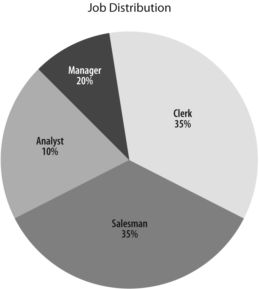
SQL> select job, count(*)
   2 from emp
   3 group by job;

JOB         COUNT(*)
--------- ----------
CLERK              4
SALESMAN           4
PRESIDENT          1
MANAGER            3
ANALYST            2
If you had many more rows on which to base the distribution of the test data, you could directly use the output of such a query. With just 14 rows, it is probably wiser to use the preceding result as a mere starting point. Letâs ignore the coveted job of president for the time being; it will always be possible to manually update one row later. What I want is the distribution of data shown in Figure 4-1.
Generating such a distribution is easy if we associate one job name to one range of values between 0 and 100: all we need to do is to generate a random number uniformly distributed in this interval. If it falls between 0 and 35, weâll return CLERK; if it falls between 35 and 70, weâll return SALESMAN; between 70 and 80, MANAGER; and between 80 and 100, ANALYST. From a practical point of view, all we need to do is compute cumulated frequencies.
Now I will show you in detail how to set this up on something more sophisticated than job names: family names. Of course, I could generate random strings, but somehow, DXGBBRTYU doesnât look like a credible surname. How can I generate a realistic-looking list of people? The answer, as is so often the case, is to search the Internet. On many government websites, you can find some statistical information that makes for wonderful data sources. If you want to generate American family names, for instance, the Genealogy section of the http://www.census.gov website is the place to start.[28] Youâll find on this site the most common American family names, with their ranking and the number of bearers.
If you want to generate a relatively small number of different names, you can download Top1000.xls, which contains the 1,000 most common American names according to the last census (a bigger, more complete file is also available if you want a larger selection of common names). Download this file and save it as a .csv file. Here are the first lines from the file:
name;rank;count;prop100k;cum_prop100k;pctwhite;pctblack;pctapi;\..
   .. (first line cont'd) ..\pctaian;pct2prace;pcthispanic
SMITH;1;2376206;1727,02;1727,02;73,35;22,22;0,40;0,85;1,63;1,56
JOHNSON;2;1857160;1349,78;3076,79;61,55;33,80;0,42;0,91;1,82;1,50
WILLIAMS;3;1534042;1114,94;4191,73;48,52;46,72;0,37;0,78;2,01;1,60
BROWN;4;1380145;1003,08;5194,81;60,71;34,54;0,41;0,83;1,86;1,64
JONES;5;1362755;990,44;6185,26;57,69;37,73;0,35;0,94;1,85;1,44
MILLER;6;1127803;819,68;7004,94;85,81;10,41;0,42;0,63;1,31;1,43
DAVIS;7;1072335;779,37;7784,31;64,73;30,77;0,40;0,79;1,73;1,58
GARCIA;8;858289;623,80;8408,11;6,17;0,49;1,43;0,58;0,51;90,81
RODRIGUEZ;9;804240;584,52;8992,63;5,52;0,54;0,58;0,24;0,41;92,70
WILSON;10;783051;569,12;9561,75;69,72;25,32;0,46;1,03;1,74;1,73
...
Although we really need the name and cumulated proportion (available here as the fifth field, cum_prop100k, or cumulated proportion per 100,000), I will use the first three fields only to illustrate how I can massage the data to get what I need.
First I will create the table name_ref as follows:
create table name_ref(name     varchar(30),
                     rank      int,
                     headcount bigint,
                     cumfreq   bigint,
                     constraint name_ref_pk primary key(name));
The key column from which to pick a name is cumfreq, which represents the cumulated frequency. For data in this column, I chose to use integer values. If these values were percentages, integers would not be precise enough, and I would need decimal values. But like the U.S. government, I am going to use âper-100,000â values instead of âper-100â values, which will provide me with enough precision to allow me to work with integers.
At this stage, I can load the data into my table using the standard commands provided by my DBMS: BULK INSERT with SQL Server, LOAD with MySQL, and the SQL*Loader utility (or external tables) with Oracle (you will find the precise commands for each DBMS in the downloadable code samples described in Appendix A).
Once the original data is loaded, I must first compute cumulated values, normalize them, and then turn cumulated values into per-100,000 values. Because my population is limited in this example to the 1,000 most common names in America, I will get cumulated frequencies that are significantly higher than the real values; this is a systemic error I could minimize by using a bigger sample (such as the list of names with more than 100 bearers, available from the same source). I can compute normalized cumulated frequencies pretty easily in two statements with MySQL:
set @freq = 0;
update name_ref
set cumfreq = greatest(0, @freq := @freq + headcount)
order by rank;
update name_ref
set cumfreq = round(cumfreq * 100000 / @freq);
Two different statements will perform the same operation with SQL Server:
declare @maxfreq real;
set @maxfreq = (select sum(headcount) from name_ref);
update name_ref
set cumfreq = (select round(sum(n2.headcount)
                            * 100000 / @maxfreq, 0)
               from name_ref n2
               where name_ref.rank >= n2.rank);
And I can do it in a single statement with Oracle:
update name_ref r1
set r1.cumfreq = (select round(100000 * r2.cumul / r2.total)
                  from (select name,
                               sum(headcount) over (order by rank
                                      range unbounded preceding) cumul,
                               sum(headcount) over () total
                        from name_ref) r2
                  where r2.name = r1.name);
The preceding code snippets represent good illustrations of syntactical variations when one treads away from the most basic SQL queries. Some of these operations (particularly in the case of SQL Server) arenât very efficient, but since this is a one-off operation on (presumably) a development database, I can indulge in a little inefficiency.
At this point, all that remains to do is to create an index on the cumfreq column that will drive my queries, and I am ready to generate statistically plausible data (if not quite statistically correct data, because I ignore the âlong tail,â or all the names outside the 1,000 most common ones). For each name I want to pick, I need to generate a random number between 0 and 100,000, and return the name associated with the smallest value of cumfreq that is greater than (or equal to) this random number.
To return one random name with SQL Server, I can run the following (using the view that calls rand()):
select top 1 n.name
from name_ref n,
     random r
where n.cumfreq >= round(r.value * 100000, 0)
order by n.cumfreq;
You can apply these techniques to generate almost any type of data. All you need is to find lists of items associated to a weight (sometimes you may find a rank, but you can create a weight from it by assigning a large weight to the first rank, then 0.8 times this weight to the second rank, then 0.8 times the weight of the second rank to the third rank, etc.). And obviously, any group by on existing data will give you what you need to seed the generation of test data that follows existing ratios.
When we want to generate test data we usually donât want a single value, but rather a large number. Inserting many random values is, surprisingly, sometimes more difficult than you might think. On MySQL, we get the expected result when we call the query that returns one random name from the select list of a query that returns several rows:
mysql> select (select name
    ->         from name_ref
    ->         where cumfreq >= round(100000 * rand())
    ->         limit 1) name
    -> from ten_rows;
+-----------+
| name      |
+-----------+
| JONES     |
| MARTINEZ  |
| RODRIGUEZ |
| WILSON    |
| THOMPSON  |
| BROWN     |
| ANDERSON  |
| SMITH     |
| JACKSON   |
| JONES     |
+-----------+
10 rows in set (0.00 sec)

mysql>
Unfortunately, SQL Server returns the same name 10 times, even with our special wrapper for the rand() function:
select (select top 1 name
        from name_ref
        where cumfreq >= round(dbo.randuniform() * 100000, 0)
        order by cumfreq) name
from ten_rows;
The following Oracle query behaves like the SQL Server query:[29]
select (select name
        from (select name
              from name_ref
              where cumfreq >= round(dbms_random.value(0, 100000)))
        where rownum = 1) name
from ten_rows;
In both cases, the SQL engine tries to optimize its processing by caching the result of the subquery in the select list, thus failing to trigger the generation of a new random number for each row. You can remedy this behavior with SQL Server by explicitly linking the subquery to each different row that is returned:
select (select top 1 name
        from name_ref
        where cumfreq >= round(x.rnd * 100000, 0)
        order by cumfreq) name
from (select dbo.randuniform() rnd
      from ten_rows) x;
This isnât enough for Oracle, though. For one thing, you may notice that with Oracle we have two levels of subqueries inside the select list, and we need to refer to the random value in the innermost subquery. The Oracle syntax allows a subquery to refer to the current values returned by the query just above it, but no farther, and we get an error if we reference in the innermost query a random value associated to each row returned by ten_rows. Do we absolutely need two levels of subqueries? The Oracle particularity is that the pseudocolumn rownum is computed as rows are retrieved from the database (or from the result set obtained by a nested query), during the phase of identification of rows that will make up the result set returned by the current query. If you filter by rownum after having sorted, the rownum will include the âordering dimension,â and you will indeed retrieve the n first or last rows depending on whether the sort is ascending or descending. If you filter by rownum in the same query where the sort takes place, you will get n rows (the n first rows from the database) and sort them, which will usually be a completely different result. Of course, it might just happen that the rows are retrieved in the right order (because either Oracle chooses to use the index that refers to rows in the order of key values, or it scans the table in which rows have been inserted by decreasing frequency). But for that to happen would be mere luck.
If we want to spur Oracle into reexecuting for each row the query that returns a random name instead of lazily returning what it has cached, we must also link the subquery in the select list to the main query that returns a certain number of rows, but in a different wayâfor instance, as in the following query:
SQL> select (select name
  2          from (select name
  3                from name_ref
  4                where cumfreq >= round(dbms_random.value(0, 100000)))
  5          where rownum = 1
  6            and -1 < ten_rows.num) ename
  7  from ten_rows
  8  /

ENAME
------------------------------
PENA
RUSSELL
MIRANDA
SWEENEY
COWAN
WAGNER
HARRIS
RODRIGUEZ
JENSEN
NOBLE

10 rows selected.
The condition on â1 being less than the number from ten_rows is a dummy conditionâitâs always satisfied. But Oracle doesnât know that, and it has to reevaluate the subquery each time and, therefore, has to return a new name each time.
But this doesnât represent the last of our problems with Oracle. First, if we want to generate a larger number of rows and join several times with the ten_rows table, we need to add a dummy reference in the select list queries to each occurrence of the ten_rows table; otherwise, we get multiple series of repeating names. This results in very clumsy SQL, and it makes it difficult to easily change the number of rows generated. But there is a worse outcome: when you try to generate all columns with a single Oracle query, you get data of dubious randomness.
For instance, I tried to generate a mere 100 rows using the following query:
SQL> select empno,
  2         ename,
  3         job,
  4         hiredate,
  5         sal,
  6         case job
  7           when 'SALESMAN' then round(rand_pack.randgauss(500, 100))
  8           else null
  9         end comm,
 10         deptno
 11  from (select 1000 + rownum * 10 empno,
 12               (select name
 13                from (select name
 14                      from name_ref
 15                      where cumfreq >= round(100000
 16                                       * dbms_random.value(0, 1)))
 17                where rownum = 1
 18                  and -1 < t2.num
 19                  and -1 < t1.num) ename,
 20               (select job
 21                from (select job
 22                      from job_ref
 23                      where cumfreq >= round(100000
 24                                       * dbms_random.value(0, 1)))
 25                where rownum = 1
 26                  and -1 < t2.num
 27                  and -1 < t1.num) job,
 28               round(dbms_random.value(100, 200)) * 10 mgr,
 29               sysdate - rand_pack.randexp(0.6) * 100 hiredate,
 30               round(rand_pack.randgauss(2500, 500)) sal,
 31               (select deptno
 32                from (select deptno
 33                      from dept_ref
 34                      where cumfreq >= round(100000
 35                                       * dbms_random.value(0, 1)))
 36                where rownum = 1
 37                  and -1 < t2.num
 38                  and -1 < t1.num) deptno
 39        from ten_rows t1,
 40             ten_rows t2)
 41  /

  EMPNO ENAME        JOB       HIREDATE         SAL       COMM     DEPTNO
------- ------------ --------- --------- ---------- ---------- ----------
   1010 NELSON       CLERK     04-SEP-07       1767                    30
   1020 CAMPBELL     CLERK     15-NOV-07       2491                    30
   1030 BULLOCK      SALESMAN  11-NOV-07       2059        655         30
   1040 CARDENAS     CLERK     13-JAN-08       3239                    30
   1050 PEARSON      CLERK     03-OCT-06       1866                    30
   1060 GLENN        CLERK     09-SEP-07       2323                    30
...
   1930 GRIMES       SALESMAN  05-OCT-07       2209        421         30
   1940 WOODS        SALESMAN  17-NOV-07       1620        347         30
   1950 MARTINEZ     SALESMAN  03-DEC-07       3108        457         30
   1960 CHANEY       SALESMAN  15-AUG-07       1314        620         30
   1970 LARSON       CLERK     04-SEP-07       2881                    30
   1980 RAMIREZ      CLERK     07-OCT-07       1504                    30
   1990 JACOBS       CLERK     17-FEB-08       3046                    30
   2000 BURNS        CLERK     19-NOV-07       2140                    30
100 rows selected.
Although surnames look reasonably random, and so do hire dates, salaries, and commissions, I have never obtained, in spite of repeated attempts, anything other than SALESMAN or CLERK for a jobâand department 30 seems to have always sucked everyone in.
However, when I wrote a PL/SQL procedure, generating each column in turn and inserting row after row, I experienced no such issue and received properly distributed, random-looking data. I have no particular explanation for this behavior. The fact that data is correct when I used a procedural approach proves that the generation of random numbers isnât to blame. Rather, itâs function caching and various optimization mechanisms that, in this admittedly particular case, all work against what Iâm trying to do.
You may have guessed from the previous chapters (and Iâll discuss this topic in upcoming chapters as well) that I consider procedural processing to be something of an anomaly in a relational context. But the reverse is also true: when we are generating a sequence of random numbers, we are in a procedural environment that is pretty much alien to the set processing of databases. We must pick the right tool for the job, and the generation of random data is a job that calls for procedures.
The downside to associating procedural languages to databases is their relative slowness; generating millions of rows will not be an instant operation. Therefore, it is wise to dump the tables you filled with random values if you want to compare with the same data several operations that change the database; it will make reloads faster. Alternatively, you may choose to use a âregularâ language such as C++ or Java, or even a powerful scripting language such as Perl, and generate a flat file that will be easy to load into the database at high speed. Generating files independently from the database may also allow you to take advantage of libraries such as the Gnu Statistical Library (GSL) for sophisticated generation of random values. The main difficulty lies in the generation of data that matches predefined distributions, for which a database and the SQL language are most convenient when your pool of data is large (as with surnames). But with a little programming, you can fetch this type of data from your database, or from an SQLite [30] or Access file.
Generating random data while preserving referential integrity may be challenging. There are few difficulties with preserving referential integrity among different tables; you just need to populate the reference tables first (in many cases, you donât even need to generate data, but rather can use the real tables), and then the tables that reference them. You only need to be careful about generating the proper proportions of each foreign key, using the techniques I have presented. The real difficulties arise with dependencies inside a table. In the case of a table such as emp, we have several dependencies:
commThe existence of a commission is dependent on the job being
SALESMAN; this relationship is easy to deal with.mgrThe manager identifier,
mgr, must be an existing employee number (ornullfor the president). One relatively easy solution if you are generating data using a procedure is to state that the manager number can be only one of the (say) first 10% of employees. Because employee numbers are generated sequentially, we know what range of employee numbers we must hit to get a manager identifier. The only difficulty that remains, then, is with the managers themselves, for which we can state that their manager can only be an employee that has been generated before them. However, such a process will necessarily lead to a lot of inconsistencies (e.g., someone with theMANAGERjob having for a manager someone with theCLERKjob in another department).
Generally speaking, the less cleanly designed your database is, the more redundant information and hidden dependencies you will get, and the more likely you will be to generate inconsistencies when populating the tables. Take the emp table, for instance. If the manager identifier was an attribute of a given job in a given department that is an attribute of the function (which it is, actually; there is no reason to update the records of employees who remain in their jobs whenever their manager is promoted elsewhere), and is not an attribute of the person, most difficulties would vanish. Unfortunately, when you refactor you have to work with what you have, and a full database redesign, however necessary it may be at times, is rarely an option. As a result, you must evaluate data inconsistencies that are likely to derive from the generation of random values, consider whether they may distort what you are trying to measure, and in some cases be ready to run a few normative SQL updates to make generated data more consistent.
Before closing the topic of data generation, I want to say a few words about a particular type of data that is on the fringe of database performance testing but that can be important nonetheless: random text. Very often, you find in databases text columns that contain not names or short labels, but XML data, long comments, or full paragraphs or articles, as may be the case in a website content management system (CMS) or a Wiki that uses a database as a backend. It may sometimes be useful to generate realistic test data for these columns, too: for instance, you may have to test whether like '%pattern%' is a viable search solution, or whether full-text indexing is required, or whether searches should be based on keywords instead.
Random XML data requires hardly any more work than generating numbers, dates, and strings of characters: populating tables that more or less match the XML document type definition (DTD) and then querying the tables and prefixing and suffixing values with the proper tags is trivial. What is more difficult is producing real, unstructured text. You always have the option of generating random character strings, where spaces and punctuation marks are just characters like any others. This is unlikely to produce text that looks like real text, and it will make text-search tests difficult because you will have no real word to search for. This is why ârandomizedâ real text is a much more preferable solution.
In design examples, you may have encountered paragraphs full of Latin text, which very often start with the words lorem ipsum.[31] Lorem ipsum, often called lipsum for short, is the generic name for filler text, designed to look like real text while being absolutely meaningless (although it looks like Latin, it means nothing), and it has been in use by typographers since the 16th century. A good way to generate lipsum is to start with a real text, tokenize it (including punctuation marks, considered as one-letter words), store it all into (guess what) an SQL table, and compute frequencies. However, text generation is slightly subtler than picking a word at random according to frequency probabilities, as we did with surnames. Random text generation is usually based on Markov chainsâthat is, random events that depend on the preceding random events. In practice, the choice of a word is based on its length and on the length of the two words just output. When the seeding text is analyzed, one records the relative lengths of three succeeding words. To choose a new word, you generate a random number that selects a length, based on the lengths of the two preceding words; then, from among the words whose length matches the length just selected, you pick one according to frequency.
I wrote two programs that you will find on this bookâs website (http://www.oreilly.com/catalog/9780596514976); instructions for their use are in Appendix B. These programs use SQLite as a backend. The first one, mklipsum, analyzes a text and generates an SQLite datafile. This file is used by the second program, lipsum, which actually generates the random text.
You can seed the datafile with any text of your choice. The best choice is obviously something that looks similar to what your database will ultimately hold. Failing this, you can give a chic classical appearance to your output by using Latin. You can find numerous Latin texts on the Web, and Iâd warmly recommend Ciceroâs De Finibus, which is at the root of the original âlorem ipsum.â Otherwise, a good choice is a text that already looks randomized when it is not, such as a teenagerâs blog or the marketing fluff of an âEnterprise Softwareâ vendor. Lastly, you may also use the books (in several languages) available from http://www.gutenberg.org. Beware that the specific vocabulary and, in particular, the character names, of literary works will give a particular tone to what you generate. Texts generated from Little Women, Treasure Island, or Paradise Lost will each have a distinct color; youâre on safer ground with abstract works of philosophy or economy.
I will say no more about the generation of test dataâbut donât forget that phase in your estimate of the time required to study how to improve a process, as it may require more work than expected.
Because refactoring involves some rewriting, when the sanity checks and light improvements you saw in Chapters Chapter 2 and Chapter 3 are not enough, you need methods to compare alternative rewrites and decide which one is best. But before comparing alternative versions based on their respective performance, we must ensure that our rewrites are strictly equivalent to the slow, initial version.[32]
Unit testing is wildly popular with methodologies often associated with refactoring; itâs one of the cornerstones of Extreme Programming. A unit is the smallest part of a program that can be tested (e.g., procedure or method). Basically, the idea is to set up a context (or âfixtureâ) so that tests can be repeated, and then to run a test suite that compares the actual result of an operation to the expected result, and that aborts if any of the tests fail.
Using such a framework is very convenient for procedural or object languages. It is a very different matter with SQL, [33] unless all you want to check is the behavior of a select statement that returns a single value. For instance, when you execute an update statement, the number of rows that may be affected ranges from zero to the number of rows in the table. Therefore, you cannot compare âone valueâ to âone expected value,â but you must compare âone state of the tableâ to âone expected state of the table,â where the state isnât defined by the value of a limited number of attributes as it could be with an instance of an object, but rather by the values of a possibly very big set of rows.
We might want to compare a table to another table that represents the expected state; this may not be the most convenient of operations, but it is a process we must contemplate.
If you are rewriting a query that returns very few rows, a glance at the result will be enough to check for correctness. The drawback of this method is that glances are hard to embed in automated test suites, and they can be applied neither to queries that return many rows nor to statements that modify the data.
The second simplest functional comparison that you can perform between two alternative rewrites is the number of rows either returned by a select statement or affected by an insert, delete, or update statement; the number of rows processed by a statement is a standard value returned by every SQL interface with the DBMS, and is available either through some kind of system variable or as the value returned by the function that calls for the execution of the statement.
Obviously, basing oneâs appraisal of functional equivalence on identical numbers of rows processed isnât very reliable. Nevertheless, it can be effective enough as a first approximation when you compare one statement to one statement (which means when you donât substitute one SQL statement for several SQL statements). However, it is easy to derail a comparison that is based solely on the number of rows processed. Using aggregates as an example, the aggregate may be wrong because you forgot a join condition and you aggregate a number of duplicate rows, and yet it may return the same number of rows as a correct query. Similarly, an update of moderate complexity in which column values are set to the result of subqueries may report the same number of rows updated and yet be wrong if there is a mistake in the subquery.
If a statement rewrite applied to the same data processes a different number of rows than the original statement, you can be certain that one of the two is wrong (not necessarily the rewrite), but the equality of the number of rows processed is, at best, a very weak presumption of correctness.
In other cases, the comparison of the number of rows processed is simply irrelevant: if, through SQL wizardry, you manage to replace several successive updates to a table with a single update, there will be no simple relationship between the number of rows processed by each original update and the number of rows processed by your version.
Comparing the number of operations is one thing, but what matters is the data. We may want to compare tables (e.g., how the same initial data was affected by the initial process and the refactored version) or result sets (e.g., comparing the output of two queries). Because result sets can be seen as virtual tables (just like views), I will consider how we can compare tables, keeping in mind that whenever I refer to a table name in the from clause, it could also be a subquery.
Before describing comparison techniques, Iâd like to point out that in many cases, not all table columns are relevant to a comparison, particularly when we are comparing different ways to change the data. It is extremely common to record information such as a timestamp or who last changed the data inside a table; if you successively run the original process and an improved one, timestamps cannot be anything but different and must therefore be ignored. But you can find trickier cases to handle when you are confronted with alternate keysâin other words, database-generated numbers (through sequences with Oracle, identity columns with SQL Server, or auto-increment columns with MySQL).
Imagine that you want to check whether the rewriting of a process that changes data gives the same result as the original slow process. Letâs say the process is applied to table T. You could start by creating T_COPY, an exact copy (indexes and all) of T. Then you run the original process, and rename the updated T to T_RESULT. You rename T_COPY to T, run your improved process, and want to compare the new state of T to T_RESULT. If you are using an Oracle database, and if some sequence numbers intervene in the process, in the second run you will have sequence numbers that follow those that were generated during the first run. Naturally, you could imagine that before running the improved process, you drop all sequences that are used and re-create them starting with the highest number you had before you ran the initial process. However, this seriously complicates matters, and (more importantly) you must remember that the physical order of rows in a table is irrelevant. That also means that processing rows in a different order is perfectly valid, as long as the final result is identical. If you process rows in a different order, your faster process may not assign the same sequence number to the same row in all cases. The same reasoning holds with identity (auto-increment) columns. Strictly speaking, the rows will be different, but as was the case with timestamps, logically speaking they will be identical.
If you donât want to waste a lot of time hunting down differences that are irrelevant to business logic, you must keep in mind that columns that are automatically assigned a value (unless it is a default, constant value) donât really matter. This can be all the more disturbing as I refer hereafter to primary key columns, as there are literally crowds of developers (as well as numerous design tools) that are honestly convinced that the database design is fine as long as there is some unique, database-generated number column in every table, called id. It must be understood that such a purposely built âprimary keyâ can be nothing but a practical shorthand way of replacing a âbusiness-significantâ key, often composed of several columns, that uniquely identifies a row. Therefore, let me clearly state that:
When I use * in the following sections, Iâm not necessarily referring to all the columns in the table, but to all the âbusiness relevantâ columns.
When I refer to primary key columns, Iâm not necessarily referring to the column(s) defined as âprimary keyâ in the database, but to columns that, from a business perspective, uniquely identify each row in the table.
One simple yet efficient way to compare whether two tables contain identical data is to dump them to operating system files, and then to use system utilities to look for differences.
At this point, we must determine how we must dump the files:
- DBMS utilities
All DBMS products provide tools for dumping data out of the database, but those tools rarely fill our requirements.
For instance, with MySQL,
mysqldumpdumps full tables; as you have seen, in many cases we may have a number of different values for technical columns and yet have functionally correct values. As a result, comparing the output ofmysqldumpfor the same data after two different but functionally equivalent processes will probably generate many false positives and will signal differences where differences donât matter.SQL Serverâs
bcpdoesnât have the limitations ofmysqldump, because with thequeryoutparameter it can output the result of a query;bcpis therefore usable for our purpose.Oracle, prior to Oracle 10.2, was pretty much in the same league as MySQL because its export utility,
exp, was only able to dump all the columns of a table; contrary tomysqldump, the only output format was a proprietary binary format that didnât really help the âspot the differencesâ game. Later versions indirectly allow us to dump the result of a query by using the data pump utility (expdp) or by creating an external table of typeoracle_datapumpas the result of a query. There are two concerns with these techniques, though: the format is still binary, and the file is created on the server, sometimes out of reach of developers.To summarize, if we exclude
bcp, and in some simple casesmysqldump, DBMS utilities are not very suitable for our purpose (to their credit, they werenât designed for that anyway).- DBMS command-line tools
Running an arbitrary query through a command-line tool (
sqlplus, mysql, orsqlcmd) is probably the simplest way to dump a result set to a file. Create a file containing a query that returns the data you want to check, run it through the command-line utility, and you have your data snapshot.
The snag with data snapshots is that they can be very big; one way to work around storage issues is to run the data through a checksumming utility such as md5sum. For instance, you can use a script such as the following to perform such a checksum on a MySQL query:
#
#   A small bash-script to checksum the result
#   of a query run through mysql.
#
#   In this simplified version, connection information
#   is supposed to be specified as <user>/<password>:<database>
#
#   An optional label (-l "label") and timestamp (-t)
#   can be specified, which can be useful when
#   results are appended to the same file.
#
usage="Usage: $0 [-t][-l label] connect_string sql_script"
#
ts=''
while getopts "tl:h" options
do
  case $options in
    t )  ts=$(date +%Y%m%d%H%M%S);;
    l )  label=$OPTARG;;
    h )  echo $usage
         exit 0;;
    \? ) echo $usage
         exit 0;;
    * )  echo $usage
         exit 1;;
  esac
done
shift $(($OPTIND - 1))
user=$(echo $1 | cut -f1 -d/)
password=$(echo $1 | cut -f2 -d/ | cut -f1 -d:)
database=$(echo $1 | cut -f2 -d:)
mysum=$(mysql -B --disable-auto-rehash -u${user} -p${password} \
       -D${database} < $2 | md5sum | cut -f1 -d' ')
echo "$ts       $label  $mysum"
On a practical note, beware that MD5 checksumming is sensitive to row order. If the table has no clustered index, a refactored code that operates differently may cause the same data set to be stored to a table in a different row order. If you want no false positives, it is a good idea to add an order by clause to the query that takes the snapshot, even if it adds some overhead.
There is an obvious weakness with checksum computation: it can tell you whether two results are identical or different, but it wonât tell you where the differences are. This means you will find yourself in one of the following two situations:
You are very good at âformal SQL,â and with a little prompting, you can find out how two logically close statements can return different results without actually running them (9 times out of 10, it will be because of null values slipping in somewhere).
You still have to hone your SQL skills (or youâre having a bad day) and you need to actually âseeâ different results to understand how you can get something different, in which case a data dump can harmoniously complement checksums when they arenât identical (of course, the snag is that you need to run the slow query once more to drill in).
In short, you need different approaches to different situations.
Using a command-line utility to either dump or checksum the contents of a table or the result of a query presumes that the unit you are testing is a full program. In some cases, you may want to check from within your refactored code whether the data so far is identical to what would have been obtained with the original version. From within a program, it is desirable to be able to check data using either a stored procedure or an SQL statement.
The classical SQL way to compare the contents of two tables is to use the except set operator (known as minus in Oracle). The difference between tables A and B is made of the rows from A that cannot be found in B, plus the rows from B that are missing from A:
(select * from A
 except
 select * from B)
union
(select * from B
 except
 select * from A)
Note that the term âmissingâ also covers the case of âdifferent.â Logically, each row consists of the primary key, which uniquely identifies the row, plus a number of attributes. A row is truly missing if the primary key value is absent. However, because in the preceding SQL snippet we consider all the relevant columns, rows that have the same primary key in both tables but different attributes will simultaneously appear as missing (with one set of attributes) from one table and (with the other set of attributes) from the other table.
If your SQL dialect doesnât know about except or minus (which is the case with MySQL[34]), the cleanest implementation of this algorithm is probably with two outer joins, which requires knowing the names of the primary key columns (named pk1, pk2, ⦠pkn hereafter):
select A.*
from A
     left outer join B
          on A.pk1 = B.pk1
          ...
         and A.pkn = B.pkn
where B.pk1 is null
union
select B.*
from B
     left outer join A
          on A.pk1 = B.pk1
          ...
         and A.pkn = B.pkn
where A.pk1 is null
Now, if you consider both code samples with a critical eye, you will notice that the queries can be relatively costly. Comparing all rows implies scanning both tables, and we cannot avoid that. Unfortunately, the queries are doing more than simply scanning the tables. When you use except, for instance, there is an implicit data sort (something which is rather logical, when you think about it: comparing sorted sets is easy, so it makes sense to sort both tables before comparing them). Therefore, the SQL code that uses except actually scans and sorts each table twice. Because the tables contain (hopefully) the same data, this can hurt when the volume is sizable. A purist might also notice that, strictly speaking, the union in the query (which implicitly asks for removing duplicates and causes a sort) could be a union all, because the query is such that the two parts of the union cannot possibly return the same row. However, because we donât expect many differences (and we hope for none), it wouldnât make the query run much faster, and getting an implicitly sorted result may prove convenient.
The version of the code that explicitly references the primary key columns performs no better. As you saw in Chapter 2, using an index (even the primary key index) to fetch rows one by one is much less efficient than using a scan when operating against many rows. Therefore, even if the writing is different, the actual processing will be roughly similar in both cases.
On a site that is popular with Oracle developers (http://asktom.oracle.com/, created by Tom Kyte), Marco Stefanetti has proposed a solution that limits the scanning of tables to one scan each, but applies a group by over the union. The following query is the result of iterative and collaborative work between Marco and Tom:
select X.pk1, X.pk2, ..., X.pkn,
       count(X.src1) as cnt1,
       count(X.src2) as cnt2
from (select A.*,
             1 as src1,
             to_number(null) as src2
      from A
      union all
      select B.*,
             to_number(null) as src1,
             2 as src2
      from B) as X
group by X.pk1, X.pk2, ..., X.pkn
having count(X.src1) <> count(X.src2)
It is perhaps worth nothing that, although using union instead of union all didnât make much difference in the previous section where it was applied to the (probably very small) results of two differences, it matters here. In this case, we are applying the union to the two table scans; we canât have duplicates, and if the tables are big, there is no need to inflict the penalty of a sort.
The StefanettiâKyte method scales much better than the classical method. To test it, I ran both queries against two tables that were different by only one row. When the tables contain only 1,000 rows (1,000 and 999, to be precise), both versions run fast. However, as the number of rows increases, performance of the classic comparison method deteriorates quickly, as you can see in Figure 4-2.
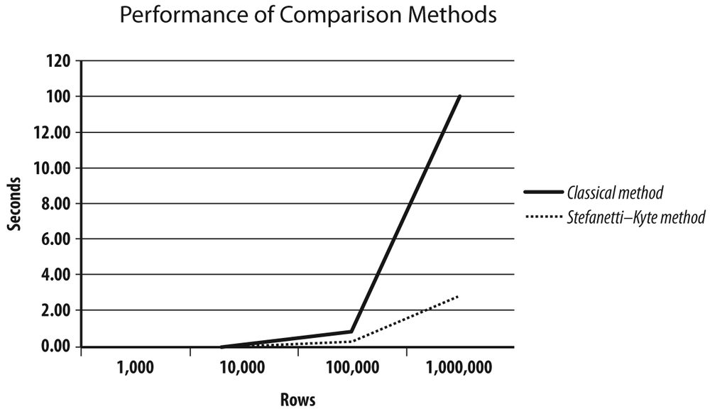
By contrast, the StefanettiâKyte method behaves much better, even against a large number of rows.
Are those comparison algorithms appropriate in a refactoring assignment? I am afraid they are more useful for comparing data once rather than for iterative testing.
Suppose that you are in the process of rewriting a poorly performing query that returns many rows. If you want to apply the preceding methods to a result set, instead of a regular table, you may want to inject the query under study as a subquery in the from clause. Unless you are very, very gifted (and definitely more gifted than I), it is unlikely that youâll hit the right way to write the query in your very first attempt. And if you have to reexecute the slow âreferenceâ query each time, it will definitely affect the time you need to reach a satisfying result. Therefore, it may be a good idea to create a result_ref table that stores the target result set:
create table result_ref
as (slow query)
Alternatively, and particularly if the expected result set is very large and storage is a concern, you may want to checksum this result setâfrom within SQL. MySQL provides a checksum table command, but this is a command for checking data integrity that applies to tables, not queries, and anyway, it provides no option to exclude some columns. All products do, however, provide a function to checksum data: MySQL has an md5() function, Oracle has dbms_crypto.hash(), and SQL Server provides hashbytes(), the latter two of which let us use either the MD5 or the SHA1 algorithm.[35] Actually, some products provide several functions for generating hash values (SQL Server also provides checksum() and Oracle provides dbms_utility.get_hash_value()), but you must be careful about the function you use. Different hashing functions have different properties: a function such as checksum() is mainly designed to help build hash tables, whereas collisions, which mean several strings hashing into the same value, are acceptable to some extent. When you build hash tables, what matters most is the speed of the function. If we want to compare data, though, the odds of having different data hashing into the same value must be so small as to be negligible, which means that we must use a stronger algorithm such as MD5 or SHA1.
There is a snag: all those functions (except for SQL Serverâs checksum_aggr(), which is rumored to be a simple binary exclusive or [XOR] operation) are scalar functions: they take a string to checksum as an argument, and they return a hash value. They donât operate on a set of rows, and you cannot pipe the result of a query into them as you can with md5sum, for instance. What would really be useful is a function that takes as an argument the text of an arbitrary query, and returns a checksum of the data set returned by this queryâfor instance, a function that would allow us to write the following:
set mychecksum = qrysum('select * from transactions');The result could be compared to a previous reference checksum, and a lengthy process could be aborted as soon as one difference is encountered. To reach this goal and write such a function, we need features that allow us to do the following:
The first bullet point refers to dynamic SQL. Oracle provides all required facilities through the dbms_sql package; SQL Server and MySQL are slightly less well equipped. SQL Server has sp_executesql, as well as stored procedures such as sp_describe_cursor_columns that operates on cursors, which are in practice handlers associated to queries. But as with MySQL, if we can prepare statements from an arbitrary string and execute them, unless we use temporary tables to store the query result, we cannot loop on the result set returned by a prepared statement; we can loop on a cursor, but cursors cannot directly be associated to an arbitrary statement passed as a string.
Therefore, I will show you how to write a stored procedure that checksums the result of an arbitrary query. Because I presume that you are interested in one or, at most, two of the products among the three I am focusing on, and because I am quickly bored by books with long snippets of a code for which I have no direct use, I will stick to the principles and stumbling blocks linked to each product. You can download the full commented code from OâReillyâs website for this book, and read a description of it in Appendix A.
Letâs start writing a checksum function with Oracle, which provides all we need to dynamically execute a query. The sequence of operations will be as follows:
Create a cursor.
Associate the text of the query to the cursor and parse it.
Get into a structure a description of the columns or expressions returned by the query.
Allocate structures to store data returned by the query.
At this stage, we run into our first difficulty: PL/SQL isnât Java or C#, and dynamic memory allocation is performed through âcollectionsâ that are extended. It makes the code rather clumsy, at least for my taste. The data is returned as characters and is concatenated into a buffer. The second difficulty we run into is that PL/SQL strings are limited to 32 KB; past this limit, we must switch to LOBs. Dumping all the data to a gigantic LOB and then computing an MD5 checksum will cause storage issues as soon as the result set becomes big; the data has to be temporarily stored before being passed to the checksum function. Unfortunately, the choice of using a checksum rather than a copy of a table or of a result set is often motivated by worries about storage in the first place.
A more realistic option than the LOB is to dump data to a buffer by chunks of 32 KB and to compute a checksum for each buffer. But then, how will we combine checksums?
An MD5 checksum uses 128 bits (16 bytes). We can use another 32 KB buffer to concatenate all the checksums we compute, until we have about 2,000 of them, at which point the checksum buffer will be full. Then we can âcompactâ the checksum buffer by applying a new checksum to its content, and then rinse and repeat. When all the data is fetched, whatever the checksum buffer holds is minced through the MD5 algorithm a last time, which gives the return value for the function.
Computing checksums of checksums an arbitrary number of times raises questions about the validity of the final result; after all, compressing a file that has already been compressed sometimes makes the file bigger. As an example, I ran the following script, which computes a checksum of a Latin text by Cicero and then loops 10,000 times as it checksums each time the result of the previous iteration. In a second stage, the script applies the same process to the same text from which I just removed the name of the man to whom the book is dedicated, Brutus.[36]
checksum=$(echo "Non eram nescius, Brute, cum, quae summis ingeniis
exquisitaque doctrina philosophi Graeco sermone tractavissent, ea
Latinis litteris mandaremus, fore ut hic noster labor in varias
reprehensiones incurreret. nam quibusdam, et iis quidem non admodum
indoctis, totum hoc displicet philosophari. quidam autem non tam id
reprehendunt, si remissius agatur, sed tantum studium tamque multam
operam ponendam in eo non arbitrantur. erunt etiam, et ii quidem eruditi
Graecis litteris, contemnentes Latinas, qui se dicant in Graecis legendis
operam malle consumere. postremo aliquos futuros suspicor, qui me ad alias
litteras vocent, genus hoc scribendi, etsi sit elegans, personae tamen et
dignitatis esse negent." | md5sum | cut -f1 -d' ')
echo "Initial checksum      : $checksum"
i=0
while [ $i -lt 10000 ]
do
  checksum=$(echo $checksum  | md5sum | cut -f1 -d' ')
  i=$(( $i + 1 ))
done
echo "After 10000 iterations: $checksum"

checksum=$(echo "Non eram nescius, cum, quae summis ingeniis
exquisitaque doctrina philosophi Graeco sermone tractavissent, ea
Latinis litteris mandaremus, fore ut hic noster labor in varias
reprehensiones incurreret. nam quibusdam, et iis quidem non admodum
indoctis, totum hoc displicet philosophari. quidam autem non tam id
reprehendunt, si remissius agatur, sed tantum studium tamque multam
operam ponendam in eo non arbitrantur. erunt etiam, et ii quidem eruditi
Graecis litteris, contemnentes Latinas, qui se dicant in Graecis legendis
operam malle consumere. postremo aliquos futuros suspicor, qui me ad alias
litteras vocent, genus hoc scribendi, etsi sit elegans, personae tamen et
dignitatis esse negent." | md5sum | cut -f1 -d' ')
echo "Second checksum       : $checksum"
i=0
while [ $i -lt 10000 ]
do
  checksum=$(echo $checksum  | md5sum | cut -f1 -d' ')
  i=$(( $i + 1 ))
done
echo "After 10000 iterations: $checksum"
The result is encouraging:
$ ./test_md5
Initial checksum      : c89f630fd4727b595bf255a5ca762fed
After 10000 iterations: 1a6b606bb3cec62c0615c812e1f14c96
Second checksum       : 0394c011c73b47be36455a04daff5af9
After 10000 iterations: f0d61feebae415233fd7cebc1a412084
The first checksums are widely different, and so are the checksums of checksums, which is exactly what we need.
You will find the code for this Oracle function described in Appendix A. I make it available more as a curiosity (or perhaps as a monstrosity) and as a PL/SQL case study, for there is one major worry with this function: although it displayed a result quickly when applied to a query that returns a few thousand rows, it took one hour to checksum the following when I was using the two-million-row table from Chapter 1:
select * from transactions
If I can admit that computing a checksum takes longer than performing a simpler operation, my goal is to be able to iterate tests of alternative rewrites fast enough. Therefore, I have refactored the function and applied what will be one of my mantras in the next chapter: itâs usually much faster when performed, not only on the server, but also inside the SQL engine.
One of the killer factors in my function is that I return the data inside my PL/SQL code and then checksum it, because I am trying to fill a 32 KB buffer with data before computing the checksum. There is another possibility, which actually makes the code much simpler: to directly return a checksum applied to each row.
Remember that after parsing the query, I called a function to describe the various columns returned by the query. Instead of using this description to prepare buffers to receive the data and compute how many bytes may be returned by each row, I build a new query in which I convert each column to a character string, concatenate their values, and apply the checksumming function to the resultant string inside the query. For the from clause, all I need to do is write the following:
... || ' from (' || original_query || ') as x'At this stage, instead of painfully handling inside my function every column from each and every row returned by my query, I have to deal with only one 16-byte checksum per row.
But I can push the same logic even further: instead of aggregating checksums in my program, what about letting the aggregation process take place in the SQL query? Aggregating data is something that SQL does well. All I need to do is create my own aggregate function to combine an arbitrary number of row checksums into an aggregate checksum. I could use the mechanism I just presented, concatenating checksums and compacting the resultant string every 2,000 rows. Inspired by what exists in both SQL Server and MySQL, I chose to use something simpler, by creating an aggregate function that performs an XOR on all the checksums it runs through. Itâs not a complicated function. Itâs not the best you can do in terms of ciphering, but because my goal is to quickly identify differences in result sets rather than encoding my credit card number, itâs enough for my needs. Most importantly, itâs reasonably fast, and it is insensitive to the order of the rows in the result set (but it is sensitive to the order of columns in the select list of the query).
When I applied this function to the same query:
select * from transactions
I obtained a checksum in about 100 seconds, a factor of 36 in improvement compared to the version that gets all the data and checksums it inside the program. This is another fine example of how a program that isnât blatantly wrong or badly written can be spectacularly improved by minimizing interaction with the SQL engine, even when this program is a stored procedure. It also shows that testing against small amounts of data can be misleading, because both versions return instantly when applied to a 5,000-row result set, with a slight advantage to the function that is actually the slowest one by far.
Enlightened by my Oracle experience, I can use the same principles with both SQL Server and MySQL, except that neither allows the same flexibility for the processing of dynamic queries inside a stored procedure as Oracle does with the dbms_sql package. The first difference is that both products have more principles than Oracle does regarding what a function can decently perform, and dynamic SQL isnât considered very proper. Instead of a function, I will therefore write procedures with an out parameter, which fits my purpose as well as a function would.
With SQL Server, first I must associate the text of the query to a cursor to be described. Unfortunately, when a cursor is declared, the text of the statement associated to the cursor cannot be passed as a variable. As a workaround, the declare cursor statement is itself built dynamically, which allows us to get the description of the various columns of the query passed in the @query variable.
--
--  First associate the query that is passed
--  to a cursor
--
set @cursor = N'declare c0 cursor for ' + @query;
execute sp_executesql @cursor;
--
-- Execute sp_describe_cursor_columns into the cursor variable.
--
execute sp_describe_cursor_columns
        @cursor_return = @desc output,
        @cursor_source = N'global',
        @cursor_identity = N'c0';
The next difficulty is with the (built-in) checksum_agg() function. This function operates on 4-byte integers; the hashbytes() function and its 16-byte result (with the choice of the MD5 algorithm) far exceed its capacity. Because the XOR operates bit by bit, I will change nothing in the result if I split the MD5 checksum computed for each row into four 4-byte chunks, apply checksum_agg() to each chunk, and finally concatenate the four aggregates. The operation requires some back-bending, but it does the trick.
With MySQL, as I have already pointed out, dynamic SQL possibilities are more limited than in Oracle or SQL Server. Nevertheless, writing a procedure that checksums an arbitrary query is less difficult than it might seem. We can work around the lack of support for the dynamic description of the columns returned by a query by creating a table that has the structure of the result set (I suppose that all computed columns have an alias):
create tablesome_unlikely_nameas select * from (original query) limit 0
Note that it is create table, and not create temporary table. Because for MySQL the table is permanent, I can retrieve its descriptionâthat is, the description of the columns returned by the queryâfrom information_schema. Of course, I would not advise drive-by table creation in a production database. But in a test or performance database, I usually lower my moral standards by a number of degrees.
Knowing the names of the columns, building a query that concatenates them and applies the md5() function to the result is a piece of cake. As with SQL Server, the 16-byte MD5 checksum is too big a mouthful for the built-in bit_xor() aggregate function: it takes as an argument, and returns, a 64-bit integer. As with SQL Server, splitting MD5 checksums (in two this time) and applying bit_xor() to each part separately before gluing everything back together in the end makes the checksums more palatable.
As you have seen, there are several ways to check that a process rewrite gives the same result as the original version. Depending on whether you rewrite unitary queries or full processes, the volume of data you have to process, the speed with which you want to iterate, and the level of detail you need to help you correct potential differences, several options are possible; usually you will want to use a combination of methods, checking the number of rows there, checksumming here, and comparing data elsewhere.
Beware, though, that even the strictest comparison of data cannot replace a logical analysis of the code. Although you can prove that a proposition is false by finding one example for which it doesnât work, finding one example for which it works is no proof of truth. Because SQL is (loosely at times) based on logical concepts, exclusions, intersections, combinations of and and or conditions, plus the odd null that mischievously refuses to be either equal to or different from anything else, the proof of correctness is in the query itself. And there are even some very rare cases where correctness doesnât necessarily mean identical results.
A customer once asked me, after I presented a much faster rewrite of an initial query, whether I could prove that it gave the same result, and I was really annoyed: my query didnât return exactly the same results as the original one, on purpose. This query was the first stage in a two-stage process, and its purpose was to identify a small set of possible candidates in a fuzzy search. Because the second stage, which really identified the final result, was comparatively fast, I opted for a slightly laxer but much faster filtering in the first stage (while advocating a rethinking of the whole process). I would have gone nowhere with a strict identity of results in the first stage.
Now that we have test data and different ways to test whether rewrites apply equivalent processes to data, letâs turn our attention back to the core topic of this book: improving existing SQL applications. First, letâs consider the rewriting of slow queries, which weâll do in the following chapter.
[25] Commercial products are available for extracting consistent data sets from production databases, but unfortunately, if you are a consultant (like I am), you cannot expect all of your customers to have bought them; otherwise, the absence of referential integrity constraints may seriously hamper their capabilities.
[26] One of the pioneers of computer science and the father of one method of random number generation, John von Neumann once jocularly commented about the sinful state of people trying to produce randomness through arithmetical means.
[27] mu (μ) and sigma (Σ) are the names of the Greek letters traditionally used to represent mean and standard deviationâthat is, the measure of the spread around the mean.
[28] Wikipedia offers an article on the most common surnames for other countries: http://en.wikipedia.org/wiki/Common_surnames.
[29] On Oracle 11g at least.
[30] * SQLite is one of my favorite tools whenever I need to organize personal data, whether it is reference data, as in this case, or collected performance data.
[31] You can find examples on such a site as http://www.oswd.org, which offers open source website designs.
[32] Actually, I have seen cases when rewrites have revealed some bugs in the original code, and therefore the result was not strictly identical in the old and new versions. But we can probably ignore such unusual cases.
[33] It is worth mentioning that most unit testing frameworks available for database servers are actually designed for stored proceduresâin other words, the procedural extension of the language.
[34] Although MaxDB, available from the same provider, implements it.
[35] SHA1 is better for cryptography, but we are not trying to encrypt data, we just want to checksum it, and MD5 does the job perfectly well.
[36] To all readers who remember vaguely either Roman history or Shakespeareâs Julius Caesar: yes, that very same Brutus. Itâs a small world.
Get Refactoring SQL Applications now with the O’Reilly learning platform.
O’Reilly members experience books, live events, courses curated by job role, and more from O’Reilly and nearly 200 top publishers.

